Overview
Our lab (Macyn, Maya, Eden and Kyle) has three different experimental areas for the summer, all involving DNA!
Senior Investigative Researcher: Macyn
Hi! It’s the Senior Investigative Researcher, Macyn Rosay, of the Andresen Lab. I’ll give a somewhat brief rundown of my project: Isothermal Titration Calorimetry Studies of DNA Condensation. I have been working on this project since last summer, though I have previously worked with fellow lab member, Aubrie Hetherington, and have made a lot of progress! In this project, I hope to condense both linear and plasmid DNA with an inorganic salt called Cobalt Hexammine, which interacts electrostatically with the negatively charged DNA. Since DNA carries a negative charge, it does not want to stick together. Thankfully, the Cobalt Hexammine has enough of a positive ion charge that counteracts the DNA’s negative charge and forces it to clump together. The purpose of this project is to watch the full two stages of DNA condensation as they happen. I do this by monitoring the temperature changes in DNA as the salt gets mixed in. By condensing the DNA, we will hopefully get a better understanding of the physics behind this process, as it has not fully been studied before.
Currently, I am using DNA from salmon testes, which is my favorite thing to mention whenever I tell anyone about my research.

This DNA is linear, which means it is the same kind that we have in our cells! However, the salmon DNA is a lot shorter than the DNA that we typically have in our cells. One of the next steps in my project is to use DNA of different lengths to see how that could impact the condensation process, which I am very excited to see! I will also be experimenting with another kind of DNA called plasmid DNA. Unlike linear DNA, plasmid DNA is circular and is typically found in bacteria, and I give a huge shout out to the Buettner Lab for graciously donating some of their supply!
The machine that I use to do most of my experiments is called the Isothermal Titration Calorimeter, or the ITC. The machine has two cells. One is the reference cell, which just has water. The other cell, the sample cell, holds our DNA samples. The ITC keeps both cells at the same temperature. Then, a syringe gets loaded up with our salt sample, which gets pushed into the sample cell.

As our salt slowly gets injected into the DNA, the ITC will measure the change in the DNA’s temperature by comparing it to the constant temperature of the water. Basically, the ITC uses the water cell to measure the temperature of the DNA. The data from this looks like a bunch of sharp peaks that gradually get smaller and then finally will flip as the DNA condensation is fully finished.

This project has definitely been an uphill battle as I am constantly adjusting the concentration of the salt samples and analyzing the data as it comes in. However, I have had a lot of fun with it and am very excited to see where it goes!
On the Computer: Maya
I (Maya) am taking a computational analysis approach to ion competition and DNA. Before I began running simulations, I had to gain an initial understanding of the experiments, as well as the programs I would be using to test them. As a physics major, I had to do a lot of outside research to understand the biology aspects of DNA electrostatics. In short, I learned that different ions react differently with DNA due to varied charges. Because DNA is a negative charge, +1, +2, and +3 (etc.) ions will be uniquely attracted to the strand, and negative ions will be uniquely repulsed. In my experiments, we simulate a strand of DNA in a 9 x 15 x 15 nanometer box of water and add different concentrations of sodium (+1 charge), cobalt hexamine (+3), and chlorine (-1).
Using Linux, I implement the Gromacs program to run these simulations. Gromacs is a program used specifically for molecular dynamics of proteins and nucleic acids using inputs and outputs. After a tutorial and plenty of practice simulations, I am now running a plethora of simulations with different values of sodium, cobalt hexamine, and chlorine. We are looking at two specific results from this data: the bound concentration and bulk concentrations. The bound concentration is a radial integration value of the number of ions that surround the DNA on average over time, while the bulk concentration is the average number of ions that exist further away from the DNA, when it is not attached to it. To achieve these values, I put the simulations into Python for graphical and numerical analysis.
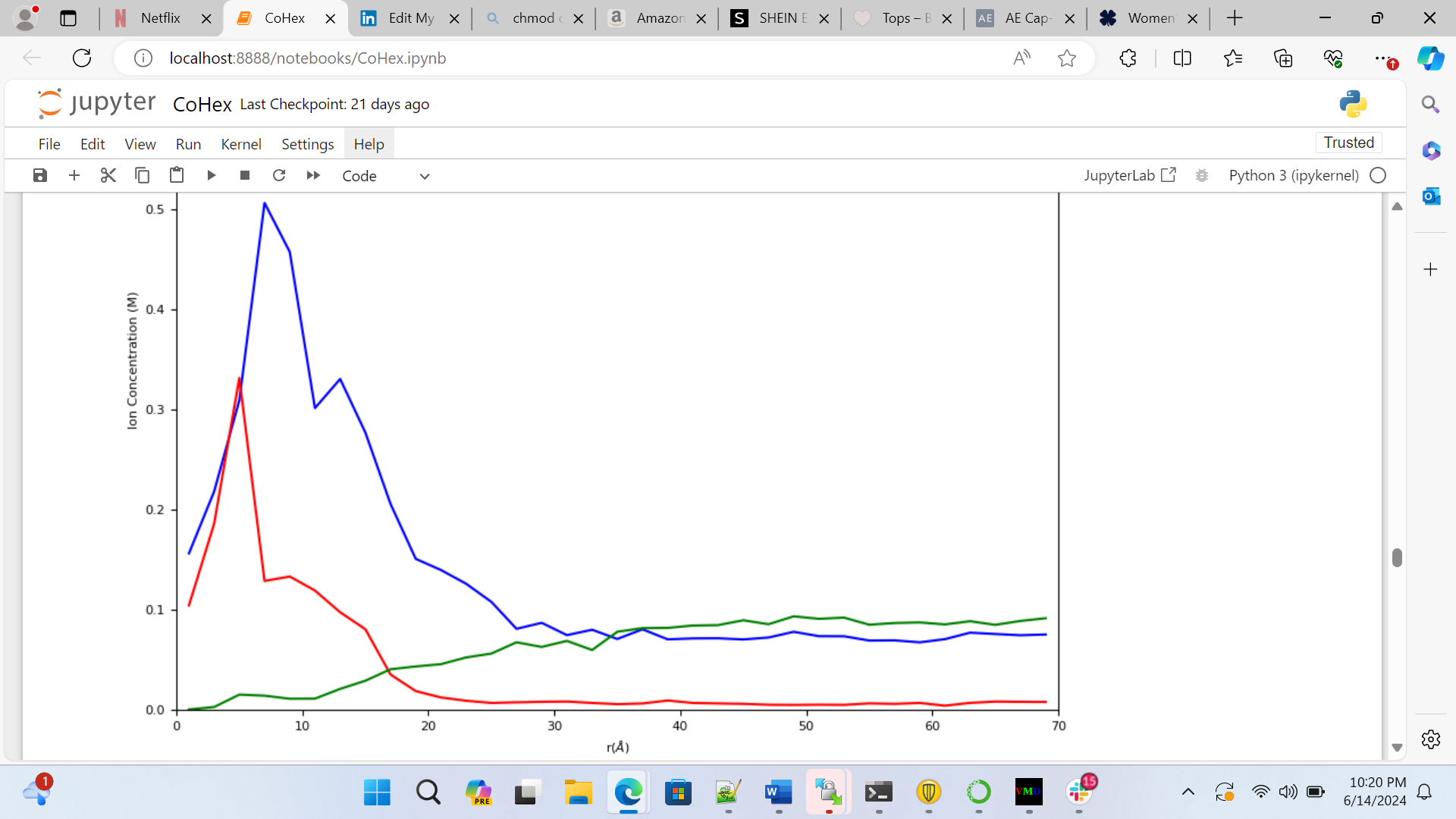

In Figure 1, we can see the bound concentration is the value of the area under the peaks closest to the DNA, while the bulk concentration is the value where the concentration levels out. In Python, we can find exact values for both of these numbers. My and Andresen’s goal, however, is to analyze the competition between the +1 and +3 ions and their resulting bulk concentrations and create an equation that can predict the bulk values. Currently, I am finding output bulk concentration values for sodium and cobalt hexamine depending on the input concentrations. Once we have ran enough tests, we can start considering equations that can theoretically bring the variables together.
Kyle and Eden on Nucleosomes & Chromatin!
When we first started our research this summer we were working on finding the best digestion for our chromatin. A digestion is a way to get a fragment of a larger substance, in our circumstance, we are digesting chromatin to get nucleosomes. Our Senior Investigative Researcher (SIR) Macyn Rosay helped us to begin this process and slowly got us to do the process on our own. For the past week, we have been doing the digestion on our own, where we were looking for the best time for the 15-unit digestion. In the prior week, we had done a unit digestion that led us to 15 units the best for the digestion of our chromatin (so many gels). Unit digestion is a way for us to find the baseline of Micrococcal Nuclease (MCN) to use to get the most amount of nucleosomes. From there we did a time digestion that ranged from 10 minutes to 55 minutes, and from this digestion, we concluded 30 minutes was the best for nucleosomes (see Fig. 1). Since 30 minutes was the blessed digestion we had (finally) moved to the next step which is mass digestion (only one more gel yayyyyyyyy). The digestion process will be explained more in-depth later, for now, enjoy our fluorescent gel.
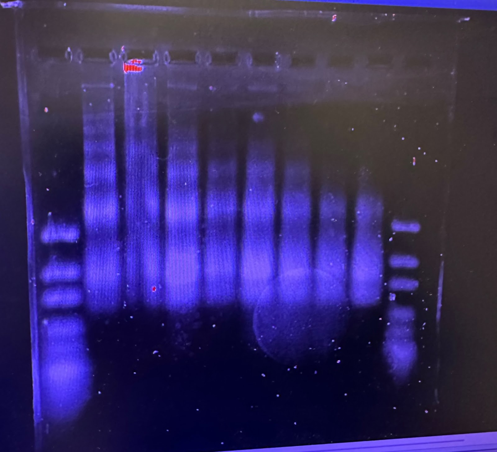
Figure 1: 15 unit Time Digestion of Chromatin
Once we (finally) made a good gel, we could move on. We spent the rest of the day digesting chromatin. We separated a sample of 50 mL of chromatin into two separate test tubes with 25 mL in each just to make sure if we mess up (which we won’t), we are not using up all of the chromatin that we already have. If we do, then it’s back to the farm to get more chicken blood!
We then added 4.5 mL of MCN to each of the two test tubes filled with chromatin and then centrifuged them. After that, we equally separated this new solution (chromatin + MCN) into 5 test tubes with 5 mL each and heated these samples for 30 minutes at 37 ℃. It was now time to make (another!) gel (and listen to Lana Del Rey of course). Once 30 minutes had passed, we combined the 5 samples and added 1.25 mL of EDTA before putting it on ice for about 10 minutes (time for more Lana).
Next, we prepared two samples for the gel, one with 5 μL of chromatin, 5 μL proteinase K, and 0.5 μL SDS. The other sample had 5 μL of digested rather than undigested chromatin. We then placed these two samples into the isotemp for 50 minutes at 50 ℃.
It was now time to move on to a higher-power centrifuge, which Professor Andresen taught us how to use. We added the digested chromatin to two centrifugal filter units and let those spin for about 10 minutes. In the meantime, we made a sample of 1.0 M NaCl which we later used to make 1.0 L of TEM buffer (Tris, EDTA, NaCl).
We then finished the digestion and loaded the gel before letting it run for about 2.5 hours. While it ran we took a lunch break at the world-renowned Bullet Hole (it is THAT good). Once they were ready, we analyzed the gels and got the thumbs up from Professor Andersen (YAY).
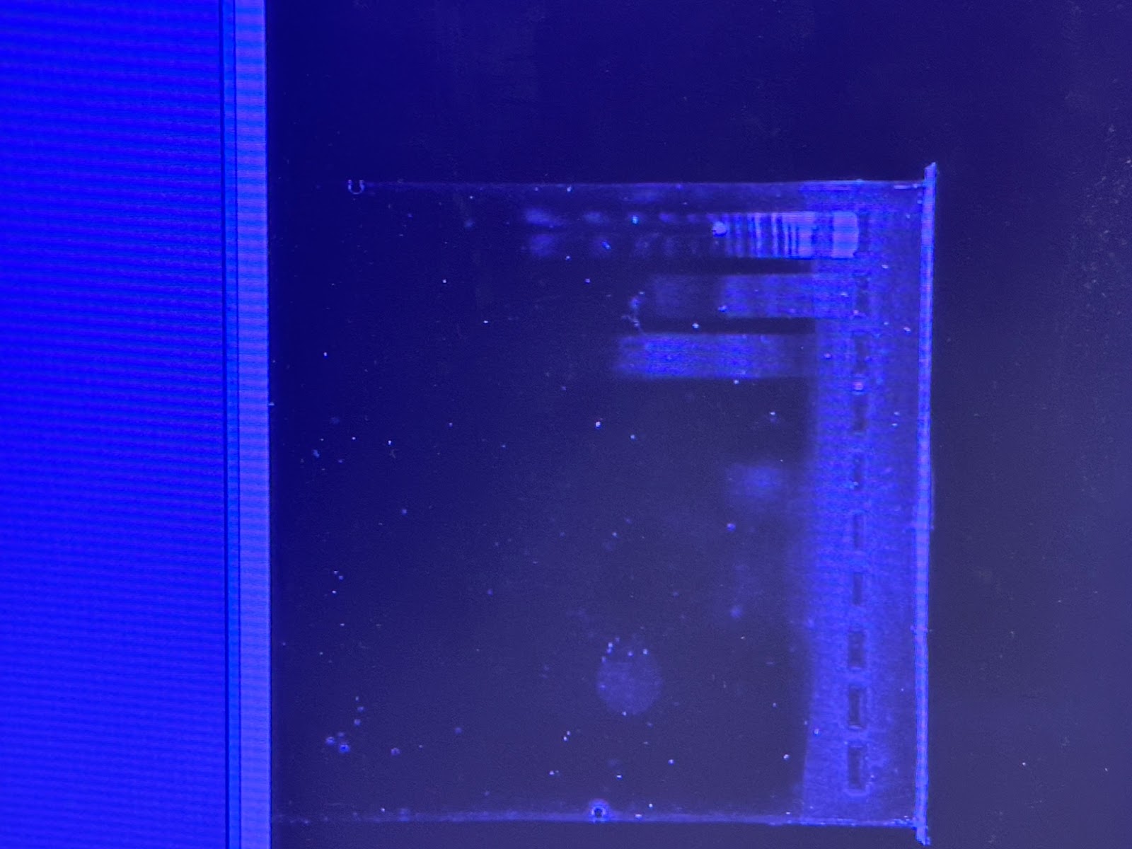
Figure 2: Digestion of Original Chromatin & 30 min Digested Chromatin
So through some rough patches in the first few weeks, we made a breakthrough, but even when we were going insane we always had great music playing.
