Hi, I’m Tom Doan. This summer, I am working with Professor Presser on Procedural Content Generation (PCG) in the Quantum Game. PCG refers to creating game content automatically, usually via artificial intelligent algorithms.
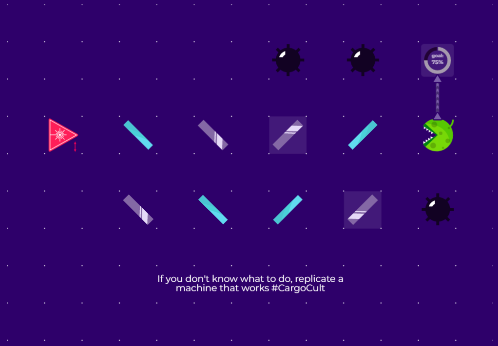
The Quantum Game In this project, we work on The Quantum Game, an online laboratory project by Quantum Flytrap team that simulates quantum mechanics phenomena interactively and intuitively. The link to the project is quantumgame.io
The landing page of the Quantum Game project at quantumgame.io
The online laboratory has two main parts, a Virtual Lab, where users have a sandbox to customize the setting of the optical table and the Quantum Game, an introduction of the simulations.
The Virtual Lab with all elementsA level in the Quantum Game with specific goalsThe two modes of the project
The game serves as an introduction to people with little to no prior exposure to quantum mechanics. As a person who only learned little about quantum mechanics in theory. I find this introduction a great way to understand the laboratory setup that illustrates quantum mechanics experiments. As I got interested in the game, I find that the game only has a limited number of levels, and I wanted to create more levels for the game; so in this research we decided to use PCG techniques to generate new levels for the game.
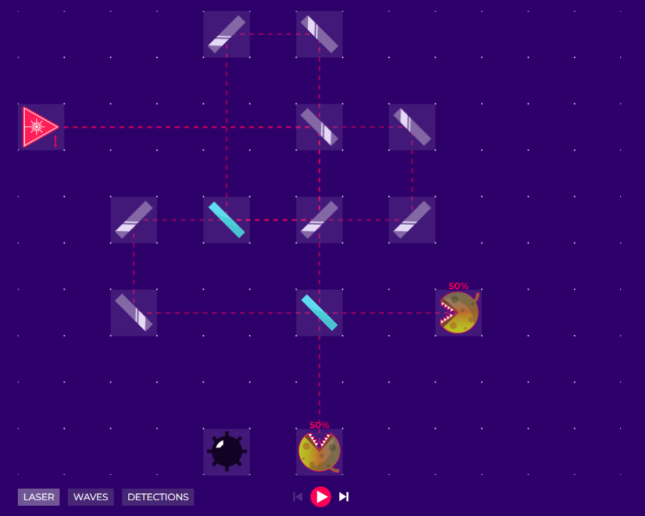
How we gonna do it The Quantum Game is grid-based, which means that the game pieces are placed in a grid order. However, in a level of the game, the structure that the player(s) build and interact with is the structure of the light ray(s). The two following pictures illustrate the grid-based setup, and the light ray(s) graph-like structure of a level of the game.
The grid-based setup of the above level
The light ray graph of the above level
In my program that generates new levels for this game, we make use of both of these ways of representation to create levels.
The approach we are taking also uses a context-free grammar (CFG) to develop light ray graphs that can be translated into grid-based setup. To generate a “good” set of levels, we also use an algorithm called evolution algorithm that can be combined with CFG, as described in the work of O’Neill and Ryan (DOI: 10.1109/4235.942529).
So far, we have created pseudocode for the project and is on track to produce the fully functional PCG for the Quantum Game by the end of this summer. Below is a level that is generated from using the pseudocode and throwing dice.
123456Hello! My name is Quentin Heise. I am a rising senior, a mathematics major, and a data science minor. This summer, I am collaborating with Professor Johnson (Physics) to continue the work Kelvin Cupay (class of 22) started two years ago. We are analyzing the card game WAR! WAR is a game that many young kids play, which involves two players with half a deck of cards each. The objective is to gain all of your opponent’s cards. On a skirmish, both players reveal the top card of their deck. The highest card wins (after 10, the ranks in ascending order are jack, queen king, and ace)! The winner of the skirmish takes both cards and puts them on the bottom of their deck. Finally, if the skirmish involves cards of equal rank, there is a special event called a WAR that begins. Players remove three cards from the top of their decks, and another skirmish occurs. The WAR does not conclude until one player wins a skirmish. Each subsequent skirmish after the first changes the war to a double war, a triple war, etc.! Once one player obtains all of their opponent’s cards, the match concludes, and the player is declared the match victor.
123456I mentioned above that WAR is a “game.” However, one can argue that WAR is not a game at all. Consider that the order in which the winner of a skirmish or WAR returns cards to the bottom of their deck is fixed (ex: ascending order). There is no randomness, and players do not have control over the order of their decks. Thus, the match victor of the “game” is determined as soon as one shuffles and deals the initial deck!
123456Before I continue, there are three vital definitions.
Win percentage is the percent of the time that a half-deck (the players’ initial decks) with specified characteristics will win.
Deck Weight is where each value (two through ace) is assigned an integer from [-6,6]. Ideally, the higher the deck weight, the higher the win percentage.
The initial advantage is the difference between the number of times both players win cards from their opponent over the first 52 cards.
For example, if player one wins ten skirmishes and player two wins 16, the players would have initial advantages of -6 and six, respectively. Unfortunately, there is ambiguity about how to take WARS into account. For example, if a player wins a triple war, they win 13 cards from their opponent (five from the first skirmish, four from both the second and third). Consider if the other player wins (a maximum of) 13 skirmishes to complete the first 52 cards. If we count the triple war as gaining the cards only once, the first player will have an initial advantage of -12. However, that player gains twice as many cards as their opponent (26 vs. 13). Furthermore, counting wars only once will reduce the initial advantage of the player that wins them. (One way I am attempting to improve the calculation of initial advantage is to exclude the matches with wars in the first round).
123456Last summer, Kelvin used Python to replicate two things from a 2006 paper by Jacob Haqqmisra [1]. These were how the win percentage correlated with deck weight and initial advantage. The correlations are nearly perfect, at 0.994 and 0.999, respectively! One might wonder why I am continuing the research this summer. I do so because many questions were previously or are currently unanswered!
123456The deck weight scale has several significant flaws. First, it does not account for when a player has cards at opposite ends of the scale. For example, if a deck has four twos and four aces, these eight cards would yield a deck weight of zero. However, the four aces are significantly better than the four twos are worse. Over 300,000 matches, the win percentage of decks with four twos and four aces is 83%! Yet, the deck weight of zero would suggest a win percentage of only 50%. I am currently experimenting with different deck weight assignments, which are all nonnegative.
123456Second, the deck weight is only usable immediately after dealing cards and before the first skirmish. This restricted use occurs by definition; one calculates deck weight over the first 26 cards only. If a player wins cards from their opponent, the earned cards are more likely to have negative values than not. Indeed, if one measures the deck weight after every skirmish, the deck weights of both players trend toward zero (the deck weight of the 52-card deck is zero).
123456Finally, I can assign deck weights to cards exponentially instead of linearly. For example, have the jack be worth 10, the queen be worth 12, the king be worth 15, and the ace be worth 20. These values would be consistent with work I did earlier this summer, where I observed that a half deck with all four aces has a win percentage of 83%. However, a half deck with all four kings only has a win percentage of 56%.
123456Another question I answered earlier this summer is how introducing randomness changes things. Previously, after winning a skirmish or war, the winner would return the cards to the bottom of their deck in a set order. Instead, I experimented with returning the cards in a random order. Interestingly, the win percentage stays the same. Things that change (increase) include the mean and average median number of games in a match and match length. I saw some that lasted over 2,000 skirmishes or WARS combined! That is a long time!
123456The final significant thing I observed is that results converge at around 60,000 matches. Comparing the results from 60,000 matches and several million matches, the differences in results are insignificant. For comprehensiveness, the results include the win percentage, the mean and standard deviation of the number of games in a match, average median and standard deviation of the number of games in a match, shortest and longest match (by the number of skirmishes and WARS combined), average starting deck weight, and average initial advantage and its standard deviation.
Raw Data
123456The left-most column is the configuration of cards in an initial 26-card deck. Either the deck is (randomly) configured to be a certain deck weight, or specific cards are in the deck. (Note that for the random configuration, there was no requirement for the half-decks). For example, “Four [9-A]s” means that the initial 26-card deck includes four nines, four tens, four jacks, four queens, four kings, and four aces. The other two cards are picked randomly from the rest of the deck. Every deck configuration was simulated in WAR games 300,000 times, except for the random deck configuration, which was simulated five million times. (Note that Professor Johnson had simulated over 100 million games last summer, but it takes a LONG time to process all that data and is borderline impossible to be thorough with limited ram and time.)
1234556Finally, the left-most column is sorted by win percentage, with the highest being at the top.
aaaaaaaaaaaaaaaaaaaaaa
a Win %
Mean # of Games in a Match
a STD of left
Median # of Games in a match
a STD of left
a Shortest Match
a Longest Match
Avg Starting Deck Weight
a Average Initial Advantage
a STD of left
Four [9-A]s
99.9
28.15
13.08
28
2.97
18
1109
78.00
24.06
2.40
Four [10, J, Q, K, A]s
98.8
37.96
43.75
31
7.41
10
1614
65.00
20.44
3.44
Four [J, Q, K, A]s
97.1
52.03
65.65
36
8.90
6
1440
52.00
16.65
4.50
Four [2, 3, Q, K, A]s
97.0
65.71
66.42
50
8.90
13
1462
13.00
4.45
4.10
Four [Q, K, A]s
94.9
70.99
85.28
45
16.31
5
1540
38.97
12.68
5.49
Four [2, 3, K, A]s
92.2
102.75
100.35
66
26.69
10
1568
0.03
0.50
5.14
Four [2, 3, 4, K, A]s
92.0
110.15
102.42
72
26.69
18
1689
-13.00
-3.68
4.13
Four [K, A]s
91.0
99.24
105.13
61
31.13
8
1628
26.03
8.59
6.28
Deck Weight 50+
87.7
105.56
119.31
56
38.55
10
1226
52.32
16.47
4.53
Four Aces
83.2
144.69
126.47
100
68.20
5
2236
12.95
4.34
6.94
Four [2, A]s
83.0
149.77
125.77
106
68.20
10
2136
-0.01
0.39
6.50
Deck Weight 45
82.3
127.59
127.98
79
66.72
10
1176
45.00
14.23
4.97
Deck Weight 40
78.4
138.32
130.79
90
75.61
10
1041
40.00
12.78
5.19
Deck Weight 35
77.0
151.44
138.53
101
84.51
8
1217
35.00
11.08
5.53
Deck Weight 30
73.5
161.07
139.38
116
94.89
6
1173
30.00
9.45
5.66
Deck Weight 25
69.5
169.80
139.09
127
99.33
10
1163
25.00
7.94
5.75
Three Aces
67.9
182.36
140.03
141
99.33
6
1789
6.49
2.19
7.16
Deck Weight 20
65.6
176.39
138.77
136
99.33
5
1248
20.00
6.31
5.91
Deck Weight 15
61.9
186.70
145.48
146
105.26
6
1476
15.00
4.89
6.10
Deck Weight 10
58.6
187.42
140.68
148
103.78
6
1486
10.00
3.22
6.08
Four Kings
55.8
186.06
142.65
146
106.75
6
2008
10.82
3.55
7.07
Deck Weight 5
54.4
192.67
143.70
152
103.78
8
1855
5.00
1.63
6.19
Deck Weight 0
50.8
192.19
139.83
152
103.78
10
1389
0.00
0.03
6.21
Two Aces
50.5
198.53
143.12
160
106.75
5
1832
0.01
0.00
7.24
Random
50.5
186.36
141.61
146
103.78
4
2277
0.00
0.00
7.48
Four Twos
46.3
187.02
141.61
146
103.78
6
1873
-13.02
-3.94
7.00
Four [2, 3]s
41.0
184.20
141.19
144
103.78
6
1761
-26.01
-7.94
6.39
Four [2, 3, 4]s
34.9
175.57
140.73
134
103.78
6
1858
-39.01
-11.97
5.62
Four [2, 3, 4, 5]s
27.4
158.33
139.33
115
97.85
8
1844
-52.02
-16.00
4.68
Four [2-6]s
18.5
127.60
131.13
75
66.72
9
1718
-65.01
-20.00
3.58
Four [2-7]s
7.2
71.82
97.78
34
11.86
18
1681
-78.00
-24.01
2.34
Four [2-8]s + Two Eights
0.0
25.45
1.38
26
0.00
18
26
-84.00
-25.84
2.01
Correlations
The correlations (R) are categorized by strength, which is determined using J. D. Evan’s scale in his 1996 book, Straightforward Statistics for the Behavioral Sciences [2]:
Very Weak:120.2 > |R|
Weak:1234560.2 ≤ |R| < 0.4
Moderate:120.4 ≤ |R| < 0.6
Strong:123450.6 ≤ |R| < 0.8
Very Strong:10.8 < |R|
a Win %
Mean # of Games in a Match
a STD of left
Median # of Games in a Match
a STD of left
Shortest Match
Longest Match
Avg Starting Deck Weight
Avg HM Advantage
Mean # of Games in a Match
-0.28 (Weak)
STD of Above
-0.20 (Weak)
0.93 (Very_Strong)
Median # of Games in a Match
-0.29 (Weak)
0.98 (Very_Strong)
0.84 (Very_Strong)
STD of Above
-0.34 (Weak)
0.98 (Very_Strong)
0.88 (Very_Strong)
0.97 (Very_Strong)
Shortest Match
-0.06 (Very_Weak)
-0.64 (Strong)
-0.65 (Strong)
-0.64 (Strong)
-0.66 (Strong)
Longest Match
0.04 (Very_Weak)
0.45 (Moderate)
0.51 (Moderate)
0.42 (Moderate)
0.36 (Weak)
-0.48 (Moderate)
Avg_Starting Deck_Weight
0.87 (Very_Strong)
-0.14 (Very_Weak)
-0.11 (Very_Weak)
-0.13 (Very_Weak)
-0.13 (Very_Weak)
-0.20 (Weak)
-0.09 (Very_Weak)
Avg HM Advantage
0.88 (Very_Strong)
-0.15 (Very_Weak)
-0.11 (Very_Weak)
-0.14 (Very_Weak)
-0.13 (Very_Weak)
-0.20 (Weak)
-0.09 (Very_Weak)
0.9999 (Very_Strong)
STD of Above
0.10 (Very_Weak)
0.82 (Very_Strong)
0.77 (Strong)
0.82 (Very_Strong)
0.76 (Strong)
-0.81 (Very_Strong)
0.58 (Moderate)
0.16 (Very_Weak)
0.16 (Very_Weak)
123456But wait, there is more! A fun game (it IS a game!) that I play with Professor Johnson and other members of my lab (and other labs occasionally) is Hacky Sack. The goal is to keep a beanbag off the ground without using one’s arms or hands. A successful “Hack” is when each person in the circle touches the beanbag at least once. As you can imagine, this is exponentially harder as more people join!
123456I am proud to say that I am the only one that has successfully “elevened” Professor Johnson this summer! “Elevening” involves hitting the beanbag between a person’s legs while their feet are flat on the ground. It is considered shameful for that person because it typically occurs when they are not paying attention! (Or they do not have proficient defenses, which is an unwritten expectation).
References
[1]1234J. Haqqmisra, “Predictability in the Game of War,” The Science Creative Quarterly, October 5, 2006.
Hi everyone and welcome to the Gownaris Lab blog post! We are spending our summer working with the US Fish and Wildlife Services (USFWS) on Petit Manan Island in the Gulf of Maine. We’ll tell you all about the work we’re doing here on the island, but first let’s start with some introductions!
Introductions
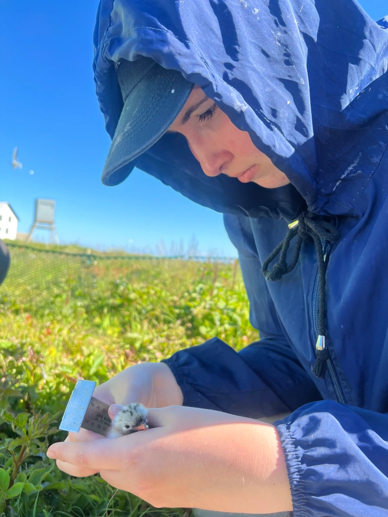
My name is Kaiulani and I am a rising senior. I am majoring in Environmental Studies and completing fieldwork this summer for my honor’s thesis. Protecting the earth and its inhabitants has always been important to me. I found an interest in ecology and in the future I would like to explore working with marine systems as well as conservation. I am so glad that Tasha brought me into her work with seabirds. I am grateful for this opportunity to spend time on not only a beautiful island, but living in a seabird colony!
Kaili measuring the wing chord of a tiny tern chick.
My name is Jehan Mody and I am a rising junior. I have majors in Environmental Studies and Biology and I will be doing my ES capstone with our research mentor, Tasha! I have been fond of animals and the natural world from a young age and hope to carry this passion into my career in the future. This passion is also why I am working with the beautiful seabirds on Petit Manan Island, protecting the seabirds’ breeding grounds and helping them to maintain healthy populations.
Jehan measuring the head length of an adult tern.
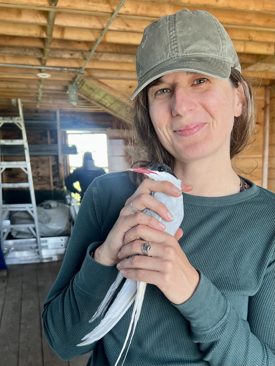
My name is Tasha Gownaris and I’m a marine ecologist and an assistant professor in the Environmental Studies department. Though I started my career working on invertebrates and fish, I fell in love with seabirds as a graduate student and haven’t looked back. This summer has been my first opportunity to bring Gettysburg College students into the field with me, and it has been such a pleasure working and living with Kaili and Jehan, in addition to the other two PMI crew members (Hallie and Nick). My research in the Gulf of Maine focuses on how seabirds adapt their foraging behavior in response to climate change – this region is warming faster than 99.5% of the ocean.
Tasha holding an adult Arctic tern.
So what exactly is the work that we’re doing here, and how does the USFWS fit in?
A tern protecting its nest.
The Gulf of Maine has an array of gorgeous islands that are home to a diversity of bird species. For some birds, these islands are a stepping stone for migrations farther north, but for some it is their final destination—thirteen species of seabird breed here over the summer. To give these birds a better chance of surviving and successfully reproducing, the USFWS manages and hires technicians to live on the islands over the summer. These lucky crew members are responsible for maintaining suitable conditions for the birds to breed in, keeping predators away, and collecting lots of data to monitor how the populations have been doing and how we can better conserve them. This summer, we are a part of the team on Petit Manan Island and are carrying out the management responsibilities of the USFWS while simultaneously collecting data for our own research projects.
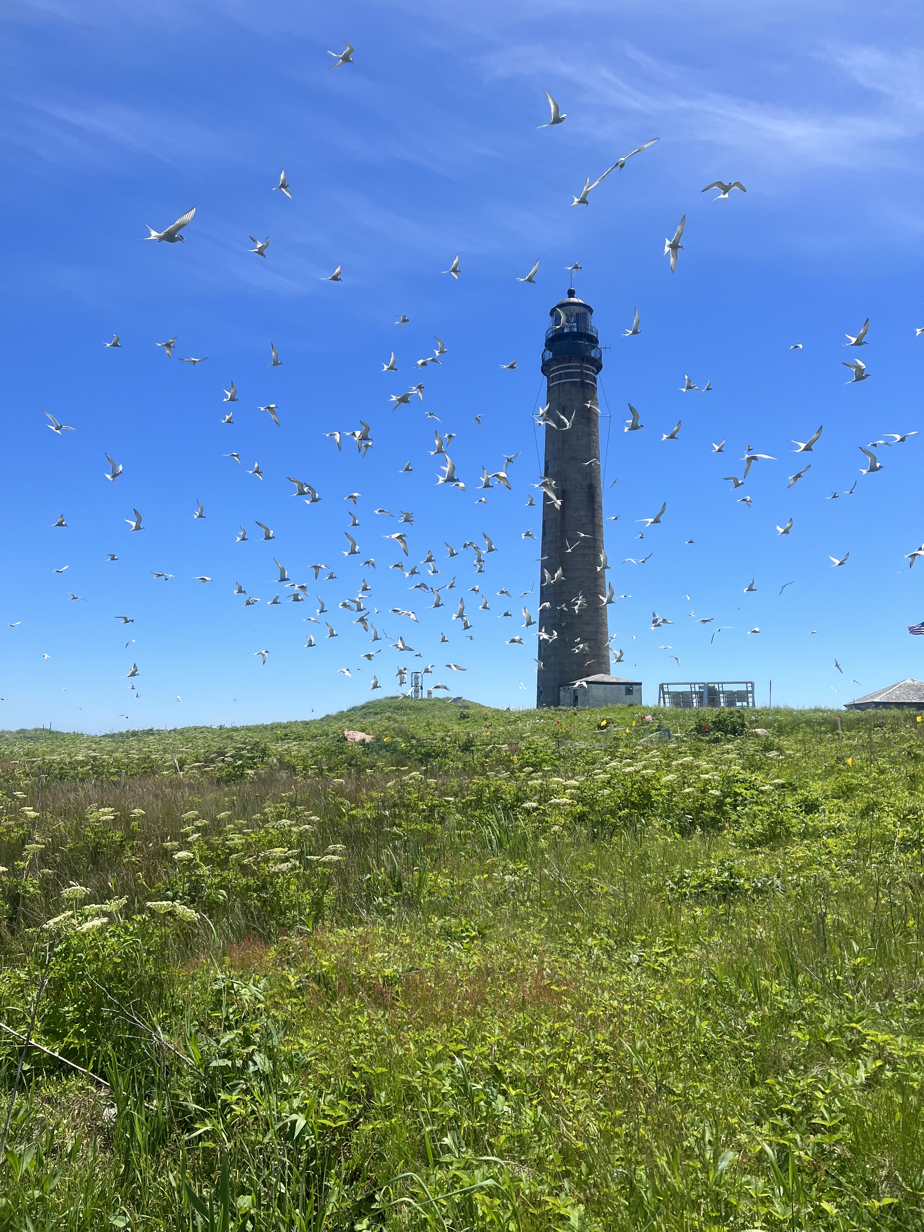
A group of terns in front of the Petit Manan Lighthouse.
But what is our life like on the island and what does all this look like on a day-to-day basis?
For starters, this is Kaiulani and Jehan’s first field season and it has been an incredible experience for them to live among a seabird colony. It was an amazing feeling to arrive here and to see all of the magnificent birds, listen to their calls surrounding us, and hear the ocean’s waves crashing on the rocky shore. On the island, we live in a house with one other member of our team, Nick, and our supervisor, Hallie. Nick and Hallie both have a ton of experience working with birds in the field, and Hallie has spent a previous season on Petit Manan Island. We are learning so much from them each and every day!
As field conditions go, you could say that our house is luxurious. We have solar power, a kitchen and dining table, a workspace, and bedrooms with actual beds and mattresses. Our bathroom is a little outhouse next to the house, with quite the view. We even have a newly installed shower with heated water! Most of our time is spent outside doing work in the field, but we like to play card games, have dinners together, and work on entering piles of hard-earned data while we’re inside.
A tiny tern chick.
We start our day bright and early at 5am and meet downstairs to brush our teeth, eat some breakfast and discuss plans for the day. Following that, we conduct provisioning stints from 6-9am on our two tern species, common terns and Arctic terns. Provisioning involves sitting in a blind and observing and recording what food the adults are bringing back, which chicks are being fed more, and the frequency at which feedings occur. It’s fun and intense and almost has a competitive edge too as we have to try to identify the prey items before they get gulped down by hungry little chicks. Kaiulani will be using our provisioning data for her research project, which she’ll talk about later.
Kaili on a provisioning watch.
After this, we take a short break and head out for our next stint, which is typically resighting. During resighting, we sit in a blind with a sighting scope and scan the area for birds that have been banded. Mostly we are focusing on Arctic terns and Atlantic puffins, but we will note bands for other species if we see them. We note down the band IDs of the birds we find and enter them into a database. These data allow USFWS and other researchers to track individual seabirds over time and to estimate their survival rates. Resighting takes a lot of patience and good eyesight, but it is also quite a relaxing and calming experience; you get to spend some time by yourself listening to and observing the birds or catching up on podcasts and music.
The view from a resighting blind.
However, we had one very interesting day of resighting that wasn’t quite as calm. Kaiulani was sitting in a blind, doing her thing, when she noticed an odd looking puffin. She came back to the house with a picture of it saying “Hey I have a weird bird, can someone ID it?” and everyone went berserk. Kaiulani had just spotted a Tufted puffin, a pacific puffin species, recording just the third observation ever of this species on the east coast and the second observation in the state of Maine. We all ran out to see it and were in complete awe and shock. It hung around for just one night, so all of the tourist boats that came full with people eager to see it the next morning were left disappointed.
A tufted puffin, in Maine!Atlantic puffins resting at puffin point
After resighting, we reconvene at the house for a quick lunch before heading back out to do our Arctic tern and common tern productivity checks. We’ve established a few plots on the island where birds are nesting and we go in every day to check how the eggs are doing and when chicks are hatching, band chicks after they’ve hatched, and measure their mass and wing chord length to calculate growth. Finding chicks in the plot is a real scavenger hunt since they hide in the vegetation and start to move around more as they grow. Their poop trails give us some hints as to where to find them and we have started to learn their favorite hiding spots. Once we do get a hold of them it usually comes with a side of poop; however, they are extremely adorable and that makes up for it all! We gather all our chicks in what we call our KFC $5 fill up bucket (below) before we process them. As a part of Tasha’s work and Jehan’s thesis, we also take blood and eggshell samples from some chicks, which we will conduct isotope analyses on. Our field season is starting to pick up since we will now start adding on productivity checks for alcids, including black guillemots and Atlantic puffins.
After our time outside, we process samples, prepare for the next day of work, and relax in the house. At 5pm, Jehan does tower count, where he goes to the top of the island’s lighthouse and surveys the shoreline and surrounding water to records counts for all the alcid species (Atlantic puffins, black Guillemots, razorbills, common murres, and common eiders). We also wash all our bird bags and put them out to dry, replenish all our kits for the next day, and finish up other small chores. By this time we’re usually in for the night and start getting ready to cook dinner. We like to sit down and eat dinner together and spend some time decompressing and chatting. We clean up for the night and are usually upstairs by 9pm to get some much needed shut eye.
What’s the plan with this data we’re collecting?
We are collecting a lot of data this summer, so there will be a lot to process when we return to Gettysburg!
Kaiulani’s Environmental Studies Capstone – My thesis will focus on the diet flexibility of Common and Arctic terns and how they cope with changes in their food supply. With an almost daily collection at a set time everyday, the provisioning data will exist at a fine temporal scale. Sea surface temperature data will also be collected from a satellite that provides daily reports on the changes of the waters around Petit Manan Island, including the foraging areas of the terns. These areas are home to hake and herring, cold water species that are preferred diet items of the terns. When the fish move farther and deeper to follow the cooler water, the terns have two options. They can spend more time foraging by following the fish that provide more nutrients, or switch to nutrient poor diet items like invertebrates. By watching these changes daily along with taking growth measurements of the chicks, I can see if the diet flexibility of the adults affects their reproductive success. My project consists of three hypotheses: the amount of preferred diet items will decrease in tern diet as sea surface temperatures rise, intraspecific variation will increase with an increase in sea surface temperatures, and finally, the individuals that maintain a provisioning diet of preferred food items will have a higher chick survival rate. We have been provisioning for a week now and we are already observing a wide variety of fish and insects, but happily seeing lots of hake and herring and some fast-growing chicks!
Jehan’s Environmental Studies Capstone – Since I am a rising junior, I still have some time to finalize what my thesis will focus on. I am using my experience in the field and the data we are collecting to formulate a study. Entering the season, I was interested in observing how individuals react to rising sea surface temperatures in their foraging behavior by looking at their stable isotope signatures. Isotope δ13C in blood serves as an indicator of foraging habitat and δ15N serves as an indicator of the trophic level of the diet. We are also collecting eggshell, prey fish, and insect/other invertebrate samples that can all be used for isotope analysis too. I have become interested in working with the eggshell data, which tells us about the diet of mom terns when they produced the eggs, and seeing whether the isotope signatures of these shells is related to chick diet, growth, or survival.
As you saw in our group photo, we get pooped on a lot! Even with daily hits on the head from the terns and the warning screams from these small but mighty birds, we are having an amazing time and learning new things every day. We hope you enjoyed learning about our summer thus far and looking at all the seabird pictures, we’ll definitely have more to add to our poster in the fall!
The sky is a strange place. My name is Braden Wolf, and I am working under Dr Johnson studying the dynamics of galaxy clusters. In other words, we are looking at how the motions of galaxies in clusters affects the modelling and observation of such celestial objects. Galaxy clusters typically have diameters between 1 and 5 Mpc, where 1 Mpc is 1 million parsecs, and 1 parsec is 3.24 light years. So, 1-5 Mpc is 3,240,000 ltyr to 16,200,000 ltyr, which is a quite significant distance. The speed of light is, by definition, 299,792,458 m/s, or 670,616,629 mph. A light year, by definition, is the distance that can be covered by light in one year. Therefore, if it takes light up to 16.2 million years to travel from one side of a galaxy cluster to the other, the galaxies in the back of the cluster can move quite a distance until their light catches up to the galaxies in the front, or even the middle of the cluster. The result is that observations of the cluster can cause galaxies to appear to be in a different location than they actually are relative to the other galaxies in the cluster. Cosmological simulations, on the other hand, do not take into account light travel time in their “snapshots” of galaxy clusters, and this leads to models that might not be quite representative of the observations that we are making of actual clusters.
Cosmological simulations model trillions of particles over the entire lifetime of the universe, using the computationally expensive n-body gravitation model, where each particle has a gravitational effect on every other particle in the simulation. Simulations such as these take a lot of data space, and therefore only release a certain number of snapshots from the runtime. For example, the simulation I am using right now, called Eagle, has released 28 snapshots over the entire life of the universe, with the snapshots being placed closer together in time as the age of the universe increases. For the 7 most recent snapshots, the time cadence is about 100 million years. Now, unfortunately, this is not quite short enough for what we are looking for, however, we are still using this simulation in order to develop the code used to analyze the data. The issue with such a long time cadence is the fact that light can travel through the entire cluster in 3-16 million years, much less than the resolution that we are able to track. In order to overcome this while we develop the analysis code, we adjust the speed of light to be 10% or even 1% of its normal value, to simulate a better time cadence between the simulation snapshots. While looking for simulations, we contacted 13 simulations, either by email or through direct website contact pages, looking for one that has a suitable time cadence. Most of the simulations are run a really high time cadences, sometimes even on the order of tens of millions of years, but due to data storage constraints, they only save a limited collection of snapshots. Some of the simulations had snapshots around 10 Myr apart, but most of them ranged around 80 to 100 Myr between snapshots.
So far in the summer, I have written code to adjust the galaxies’ position in a projection, using both velocity of the galaxies and the various snapshots recorded by the simulations. The code itself uses a couple of simple tricks to find the adjusted time model from the global time model that the simulation outputs. Originally, I used the velocity of a given galaxy and its distance from a given point in the cluster (either the closest galaxy to an observer or the center of the cluster) to find the new position of a galaxy. This method is good for a first approximation, and it can create pretty plots such as Figure 1, but it does have the disadvantage of not accounting for the acceleration of the galaxies diverting their paths, which limits the amount of statistical analysis we can do.
The second, more refined method we are using takes a galaxy’s distance from the center of mass of the cluster, which, because the speed of light is constant, allows us to compute the light travel time from the galaxy to the center of the cluster. For this test, we take the seven youngest snapshots from the simulations (22-28), and define snapshot 25 to be the one where the cluster center of mass is. Since we know the light travel time from each galaxy to the center of mass of the cluster and the time separation of each snapshot from snapshot 25, we can calculate which snapshot each galaxy is closest to. When we have that information, we can then take the position, velocity, and mass of the galaxy in that snapshot and add it to a collection of data, where all of the galaxies’ identifying information is stored. Figure 1 shows one example of this method, using 9 snapshots. The central snapshot in the diagram is snapshot 5. The goal is for each galaxy, to find which snapshot line it is closest too, and then obtain that galaxy’s physical information from that snapshot.
Figure 1: A diagram of how the projection method works, courtesy of David DeAngelo, ‘23
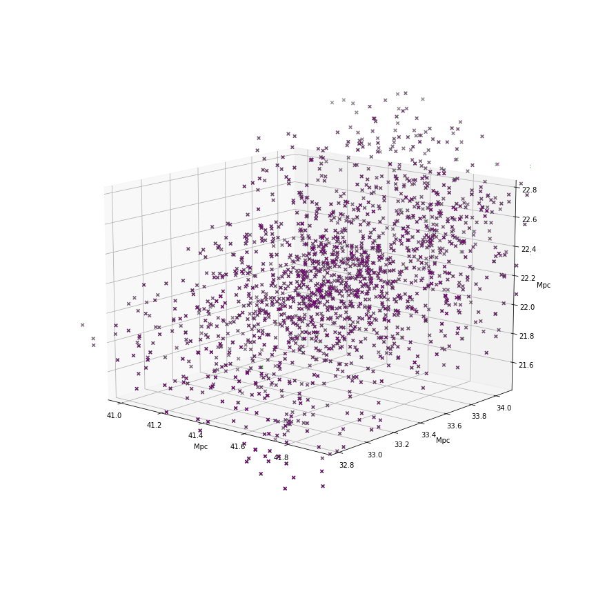
From this array, we are able to create a model of the cluster that shows both the original data (where all the galaxy position and velocity data is taken from a single snapshot) and the adjusted data (where the galaxy data is drawn from their closest snapshot). This plot for one cluster, which contains 1700 galaxies, is shown as Figure 2. This plot is derived from the velocity method.
Figure 2: Plot of a galaxy cluster, showing original and adjusted positions, using the velocity method
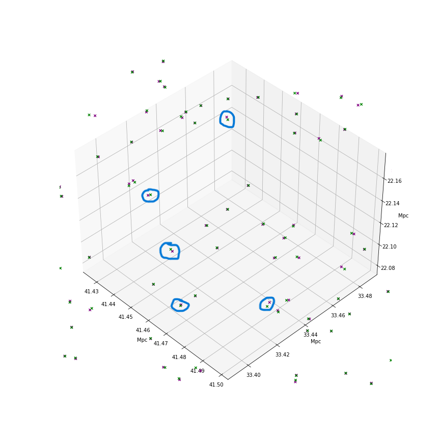
If we zoom into that plot far enough, you can actually see that the two points are plotted, one in green, and one in purple. The green point is the location of the original data, and the purple one is the new data.
Figure 3: Marked Galaxy pairs, zoomed in from Figure 2
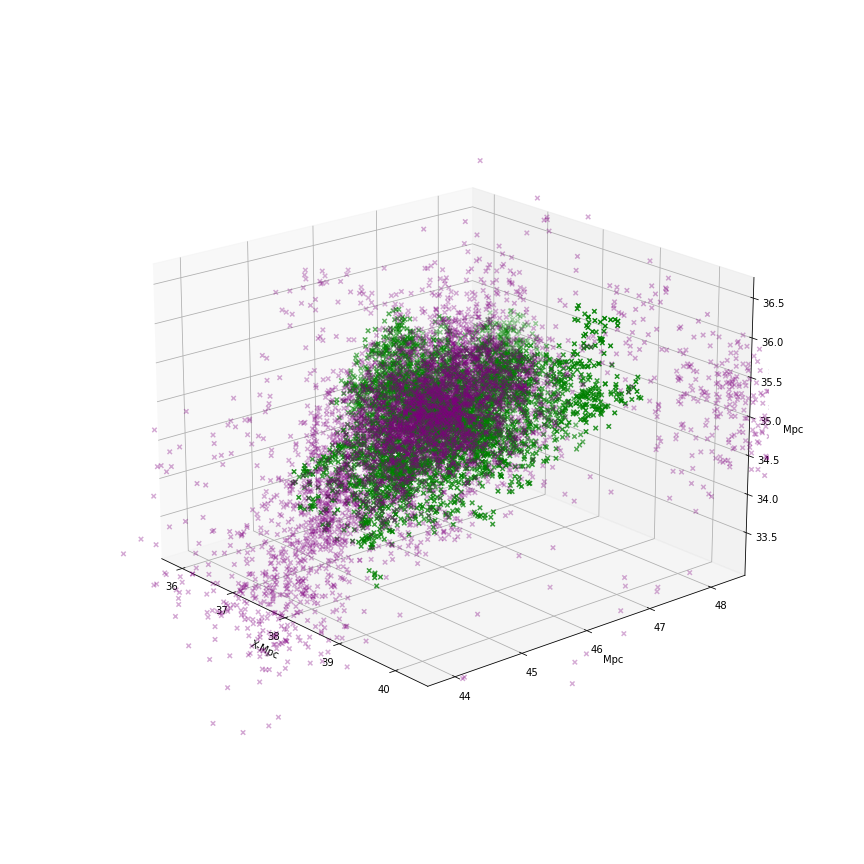
Now, Figure 4 is made using the snapshot method. This is the first time we have been able use this method to develop a plot, so there are still some revisions and optimization work to do. It takes about 2.5 hours to generate this plot. This is for a different cluster, with about 5300 galaxies. One possible explanation for the odd shape of the plot is that the cluster is moving through space, and therefore, the galaxies at different times appear to be in a different location relative to the cluster center in snapshot 25.
Figure 4: The cluster with the galaxies adjusted with the snapshot method
Once the new galaxy data is collected from the snapshot method, there are two steps that will be taken on next. First, the data will be projected cleanly onto a 2D plane, so that it would mimic the appearance of a galaxy cluster as observed from earth. Once that is complete, we can begin statistical analyses of that data and compare it to the same exact equations applied to the original dataset. We will use code written by another student to compute statistical averages of both datasets and see for a collection of clusters in the simulations if the adjusted dataset has significantly different values for those measures.
Hacky sack, of course, makes up one of the most dependable rituals of the summer. Whereas last year, I was just beginning to learn, this summer, with one year more of experience under my belt, I have found a role in the circle- lunging forwards into the center of the circle to try and keep the hack alive. Additionally, now that I have pretty much mastered the basics of the game, I can also begin to experiment with more exotic moves, which would make even more fun hacks possible. Surprisingly, the most successful hacks we have are when we are not actually paying that much attention to the circle, but rather when we are in the middle of some other conversation about a complex (or otherwise involving) topic, and we are just playing unconsciously.
Left to Right: Julianna Mendez ’23 (working for Dr. Michael Caldwell), Angelina Piette ’23, Dr. Alex Trillo, Alessandro Zuccaroli ’25
In a far away lab …
Deep in the forests of Gamboa, Panama lives the Rebel Túngara frogs who plan their next move against the Trachops Empire and their Corethrella troopers. Having won their first victory, the Túngara managed to find mates before the Empire could use their ultimate, secret weapon, ECHOLOCATION, with enough power to destroy an entire army of frogs.
Pursuing to research the Empire, the Trillo Lab races back to STRI home base with data that can save the Rebellion Túngara and restore freedom to the forest …
Male-male Túngara aggression! *cue the Star Wars theme song*
But first, where are we? An Introduction to Panama and Gamboa:
To most of the world, the Republic of Panama is best known for the Panama Canal that connects the Atlantic and Pacific Ocean. Unlike one would expect, the Atlantic Ocean borders northern Panama, whereas the Pacific Ocean lies to the South. Between these borders, Panama contains lush rainforest, teeming with the high biodiversity characteristic of the tropics.
The presence of the Panama Canal is well known. Something that the world is less likely to know, but that is just as crucial to Panama, is the indigenous population. Today, there are seven indigenous peoples in Panama, including the Wounaan, the Guna, the Emberá, the Ngäbe, the Naso Tjërdi, the Buglé, and the Bri bri. According to a 2010 census, 12 percent of the total population, or about 418,000 people identify as indigenous. These seven indigenous peoples occupy a combined 1.7 million hectares of land. Near the town of Gamboa, the Wounaan people live in the surrounding forest, and they are well-known for their craftsmanship of ancestral woven baskets, as well as their proficiency in canoes.
STRI at Gamboa, Panama
Lying close to the Panama Canal is the town of Gamboa. Gamboa is within the Canal Zone, a geopolitical border that previously denoted American owned land that extended in a radius around the Canal. The United States government left the Canal Zone on December 31st, 1999. Located within the Canal Zone, Gamboa is our home for the next couple months. Gamboa is a hub for scientific research, as it houses one of several Smithsonian Tropical Research Institute (STRI) sites in Panama. Scientists at STRI work on bats, frogs, snakes, butterflies, and much more! That said, Gamboa houses much more than STRI scientists. Many others reside in Gamboa, contributing to its quiet, welcoming atmosphere. As a result, there is a tangible sense of community, as many residents are connected by their love of conducting and sharing their research. Furthermore, the Gamboa Baking Company, operating out of a Gamboa resident’s garage-turned-kitchen, provides a great place for all members of the community to sit and relax, and even better baked goods. Also, Gamboa houses the Gamboa Rainforest Reserve, a resort that serves as a tourist attraction to many people, while some STRI employees utilize the forest near the resort to conduct research at sites such as La Chunga and La Laguna. The majority of our research is conducted in the forest of Soberania National Park, accessed via Pipeline Road. Pipeline is a hotspot for STRI scientists who all utilize the nearby, lush forest to conduct a plethora of scientific research. Each time you walk down Pipeline, you will encounter other scientists gathering data, people absorbing their surroundings while hiking, and a wide range of breathtaking wildlife.
The main interest of the Trillo lab is the effect of calling neighbors on eavesdropper attraction in frog choruses. In previous years, the Trillo lab has mainly focused on mixed-species frog choruses and heterospecific neighbors. However, this summer, the lab’s focus is to understand how attractive neighbor calls can influence the risk of predation within a single species. More specifically, the lab will be focusing on the Túngara frog and its predators: Trachops cirrhosis, or the fringe-lipped bat, and the micropredatorial Corethrella midges.
Fringed-lipped bat preying on a Túngara frog [Photo credit: A. Baugh] Ryan, Michael. (2011). Replication in Field Biology: The Case of the Frog-Eating Bat. Science (New York, N.Y.). 334. 1229-30. 10.1126/science.1214532.
For some background information, it is important to understand the intricate cost-benefit relationship associated with animal’s mating calls. While a call’s purpose is to attract females for reproduction, it also has the potential to attract eavesdropping predators. Moreover, different calls might elicit different levels of interest from eavesdroppers. Research at the Trillo lab has shown that hourglass treefrogs, which possess a less attractive call, experience an increased risk of blood-sucking midge predation when calling next to túngara frogs, which possess a more attractive call (Trillo et al, 2016, 2021). This is consistent with the Collateral Damage hypothesis, which states that attractive callers may increase the risk of predation on neighboring individuals by increasing predatory attraction to the entire aggregation. On the other hand, the Shadow of Safety hypothesis states that the more attractive caller will incur the increased risk, sheltering other less-attractive, aggregated individuals from the risk of predation. Thus, when two or more neighboring individuals utilize call types of differing attractiveness we call it asymmetric attraction (Trillo et al. 2019).
Túngara frogs in amplexus making an egg clutch with Corethrella midges swarming Provided by collaborators, Dr. Rachel Page and Dr. Ximena E. Bernal
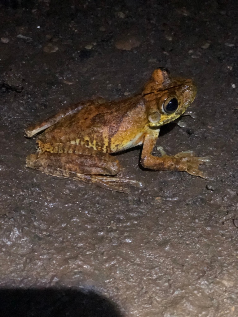
Túngara frog
The idea of collateral damage or shadow of safety across species could also be applicable within a single species, if individuals within that species use more than one type of mating call, and if one of those signals is more attractive to predators than the other. This is the case for Túngara frogs. Male túngaras have two types of calls: a simple and a complex call. The simple call consists of a single whine, whereas the complex call consists of the same whine with an additional syllable called a “chuck” at the end. These calls differ in their attractiveness to both females and predators, setting up a cost-benefit relationship. Calling simple calls poses a lesser risk of predation, but it also is less attractive to females. On the contrary, calling complex increases attractiveness to females and predators alike. These predatory interactions allow us to further investigate the Collateral Damage and Shadow of Safety hypotheses.
In nature, a solitary male túngara frog will call simple. However, in an aggregation of male túngaras, they will switch to complex calls to attract females while potentially diluting their individual risk. With this in mind, our research question this summer is: Do simple calling túngara frogs experience collateral damage or shadow of safety when calling next to a complex calling neighbor? We hypothesize that the highly attractive signaling complex calling neighbor Túngaras will increase the risk of predation and parasitism of their simple calling neighbors.
Methods of research :
Data Collection
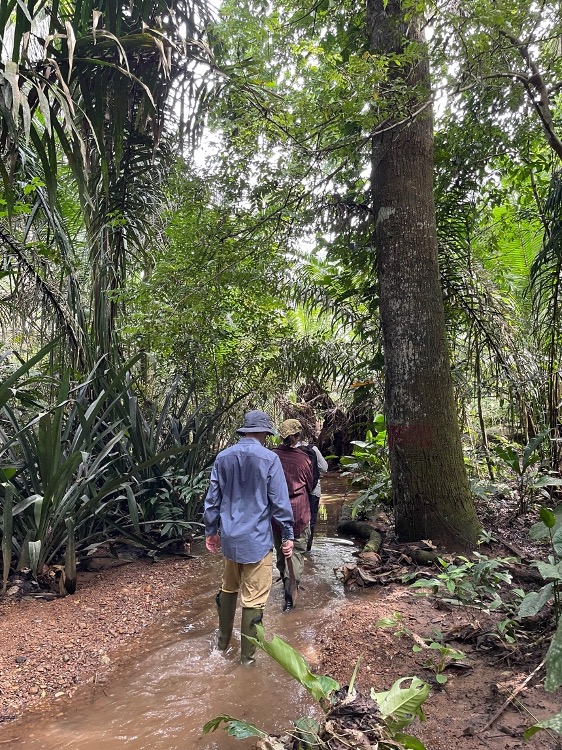
Walking through Pipeline to our site (Soberania National Park)
Our research consists of various combinations of Túngara acoustic playbacks. We set up two speakers at one of our six sites for different treatments (Simple-Simple, Simple-Silent, Complex-Complex, Complex-Silent, or Complex-Simple) in order to analyze the differences in eavesdropper predator attraction to these different types of calls in a duet.
We set up camera traps to record bats visiting each speaker, and we place fly traps above each speaker to capture the Corethrella midges attracted to each type of call.. After the experiment is done, we count the number of flies present and carefully upload the bat videos taken at each site in order to score them for bat visits. The experiments are recorded for 80 minutes.
(Warning, all our experiments are done at night, so wear your headlamps and watch out for snakes!!)
Setting up speakers
One of our resting sites at the Soberania National Park, where we wait for a trials to finish
While our trials are running, we get to wait nearby and listen to the forest. When you’re extremely quiet, you can hear some of the most amazing choruses from many different species in the silence of night.
Bat Scoring
We score bat videos blind to the treatment and use pre-determined behavioral criteria to decide whether a sighting is a bat visit to the speaker or not. A bat will visit the speaker in many unique ways: flyby (swoop down towards the speaker and swoop up), hover, or circle around the area (maybe a half circle, once, or twice) to locate the frog.Not only do we see bats in the video, but we also sometimes find really cool nocturnal species passing by the camera (and some even seem interested in the speaker!).
Midge Counting
Collecting the midges after a trial
The day after our experiments, we count how many midges were collected in each treatment (blindly as well). We use our headlamps to see the little guys stuck in the sticky glue and a pair of tweezers to count and pull them off.! Most days, we’ll count hundreds or a thousand files in a single treatment. Next time you are annoyed by a mosquito, imagine what a calling Túngara feels like!
Daily life in Panama
Most of our daily life in the tropics consists of working through all the different steps of research. From scoring bat videos, counting flies, troubleshooting with equipment, and 3-hour night hikes to run new experiments, we are constantly involved in data collection. However, on our days off, we experience some great adventures that Panama and STRI has to offer.
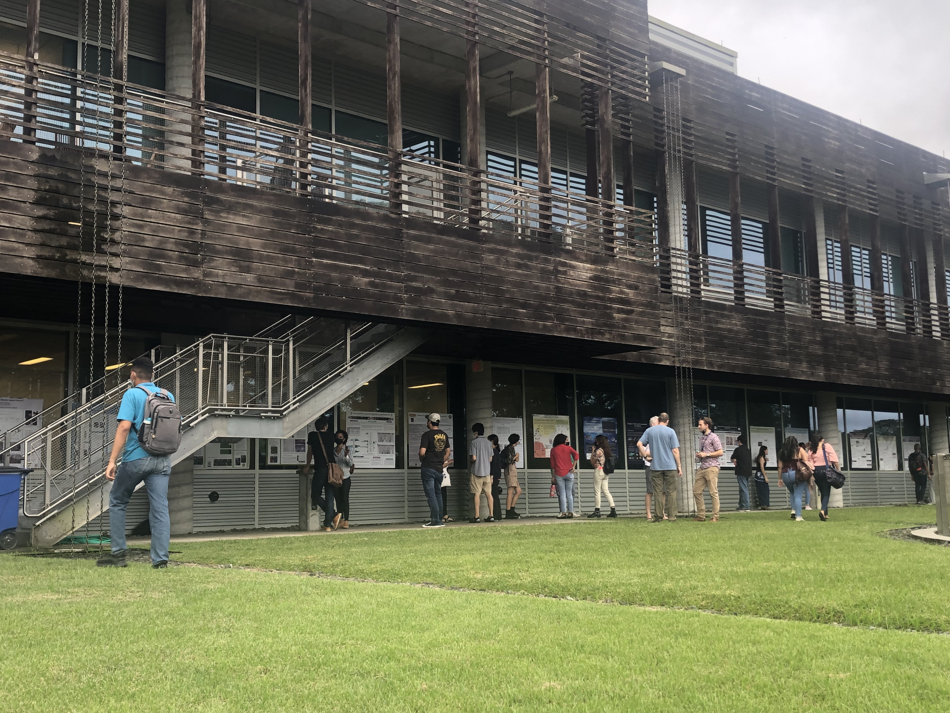
Poster session at STRI
At STRI, we have already attended several talks and we also attended a poster session that was given by the research fellows. Over 20 people presented their research and latest findings. We saw posters that focused on marine paleoethnology, botany, mammalian biodiversity, vampire bat behavior, butterfly genetics, climate change, and microbiology!
Karen Warkentin’s talk on queer perspectives in behavioral diversity studies
After the poster session, the event ended with a talk by Dr. Karen Warkentin, who discussed queer perspectives in behavioral diversity and disrupting binaries set upon by previous research. She explained how science is limited due to normalized human concepts (ie independence of gender and sex relationships) and interpretations being placed into biological studies and knowledge. Warkentin studies vibration behavior and sexual selection in frogs and she has found wide diversity and interspecific variation of communication and parental care across species.
Julianna and Alessandro at the poster session
Other times, we enjoy going on day-hikes and exploring the tropical forests. The greatest part about living in Panama is seeing new species of plants and animals everywhere you look. Species you might only see live in the zoo otherwise, here we experience naturally, in their native lands. It’s like watching a National Geographic documentary, but in real life! We’ve seen hundreds of species, from the agouti that chomp on coconuts in our backyard to the howler monkeys signaling on-coming rain. You’ll never see the same forest twice,
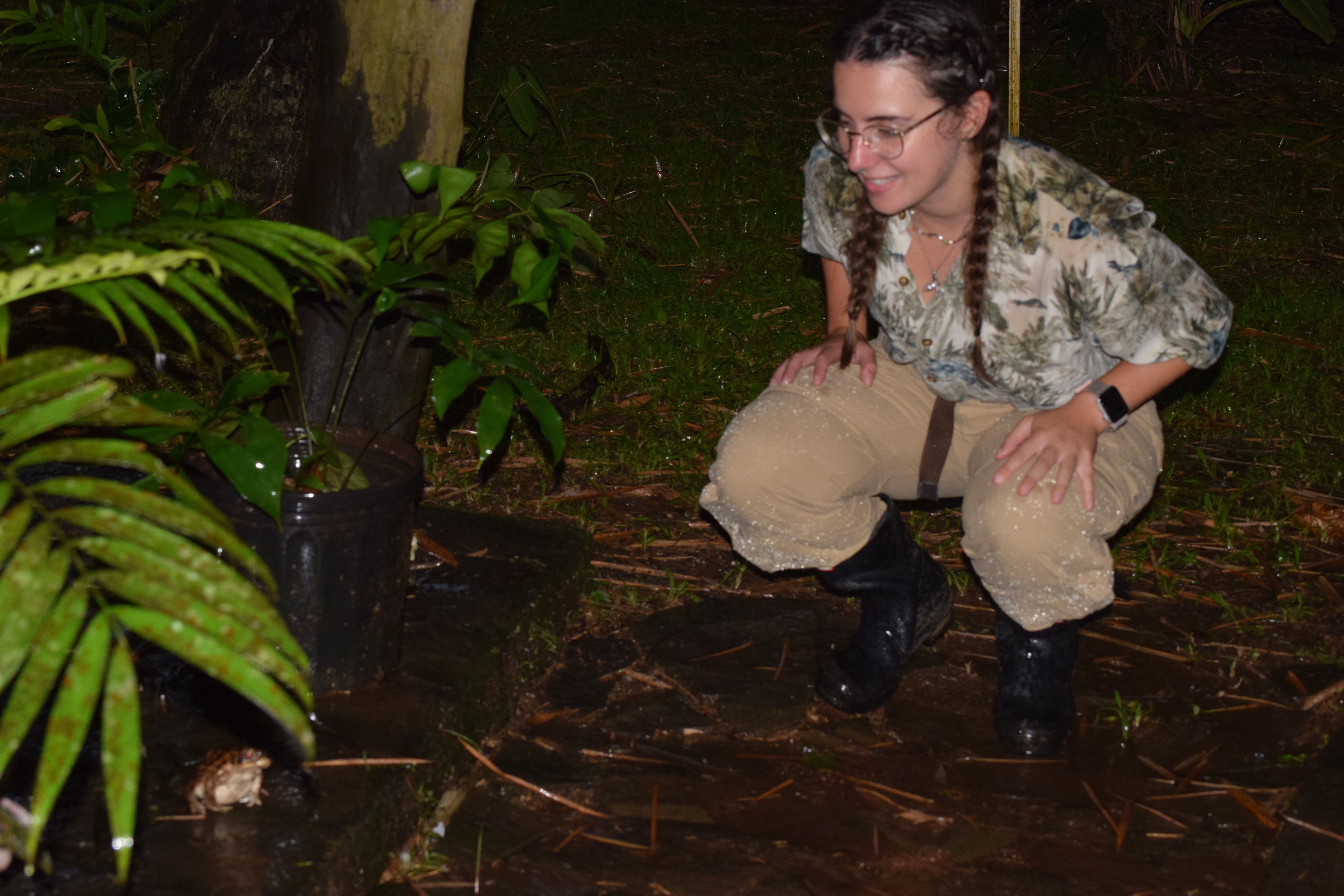
Angelina finding a cane toad in our backyard
each time we hike Soberania National Park, it changes; these forests are ever changing. And with every transformation of our surroundings come new experiences. The things you see are unique and unlike anything we’ve ever witnessed before, like an iridescent cicada hatching from her shell, a chorus of dozens of Túngara calling in the rain, a Fer-De-Lance snake curled up by our site (no worries, we were careful!), toucans flying in the distance, an ancient tree with river-like roots, just to name a few. And yet, we’ve seen barely anything compared to what these forests have to give. As one of our colleagues said, “in the rain, Panama looks like ‘Rainforest Café’ has come to life”, and I couldn’t agree with her more.
As of now, we are halfway through our time in Panama and have so much left to explore! We will continue our night hikes, discovering new species, and collecting data before our next adventure in Costa Rica, where we’ll discuss our new findings at the Animal Behavior Society Conference. We hope you enjoyed the Túngara Tavern! May the forest be with you.
Jess McThomas is a rising Junior. She is a Health Science Major with Neuroscience, Biology, and Chemistry minors. She enjoys watching criminal minds until the depths of the early morning, then coming into lab on two hours of sleep and a large iced coffee.
Everett Gillis is a rising Junior. He is a Biochemistry and Molecular Biology Major. He loves spending time jamming to heavy metal music that he listens to while hitting his newest deadlift PR.
Jenna King is a rising Junior. She is a Health Science Major with a Chemistry Minor. She is a fun-loving person that helps keep spirits high on days that do not go very well in the lab.
Dr. Jenna Craig is the mentor you wish you had. She played Basketball and received her BS in Molecular Biology at Millersville University and received her PhD in Genetics at The Pennsylvania State University. An athlete, doctor, mother, and mentor all in one. What more could you ask for!
Some Background on Bladder Cancer
Bladder cancer (BC) is often described as a heterogeneous disease in that a bladder cancer tumor consists of cells with varying molecular subtypes within a singular tumor. Bladder cancer cells are often classified according to their gene expression profiles and to their morphologies, which are physical structures observable with microscopy. These characteristics give rise to three broad categories of BC cell lines: luminal, basal, and non-type, which are referred to as molecular subtypes.
Luminal bladder cancer is a less aggressive and invasive form of BC, whereas basal bladder cancer is comparatively more aggressive and invasive, often leading to a worse patient outcome. Luminal and basal bladder cancer have opposing gene expression profiles which may cause the 5 change in aggression and invasiveness. So, what exactly is the driving force behind the differences in gene expression between the molecular subtypes?
The goal of our lab is to answer this question using various molecular biology techniques to study gene expression changes and possible regulatory mechanisms that alter the gene expression differences between luminal and basal BC. DNA methylation, the process of reducing gene expression by binding methyl groups to DNA, is a mechanism of importance in our research. We believe that DNA methylation is a major regulatory mechanism that dictates gene expression profiles of BC tumor cells and ultimately contributes to tumor heterogeneity. Forkhead Box A1 (FOXA1) has been shown to be regulated by DNA methylation specifically in basal BC. Thus, DNA methylation of FOXA1 and likely other genes, may contribute to clonal evolution of BC cells into a basal molecular subtype. In addition, because patients have far worse outcomes with basal BC, DNA methylation is likely to contribute to more aggressive and invasive forms of this disease. We hypothesize that Retinoblastoma protein 1 (RB1) is a negative regulator of aberrant DNA methylation, thus, in luminal BC cells such as UMUC1 where RB1 is expressed, FOXA1 is over-expressed.
Genetics for Dummies- some general definitions
KO (KnockOut) cells: CRISPR-Cas9 technology was used to permanently stop the expression of RB1, a tumor suppressor gene that inhibits the transcription of genes involved with cell growth. Mutations in the RB1 gene prevent it from making functional protein, making the cell unable to regulate cell division.
WT (WildType) cells: Natural cell line without any genomic manipulation.
CpG islands: Our genes have regions of repeated cytosine-guanine (CG) base pairs called CpG islands. These regions are highly susceptible to methylation of cytosines, which is critical for controlling gene expression.
FOXA1 (Forkhead Box A1): Forkhead box A1 is a transcriptional regulator and pioneer factor, making its effects on the genome as precise as the regulation of single gene expression and as broad as the unwinding of heterochromatin
RB1 (Retinoblastoma Protein 1: Retinoblastoma protein 1 is a cell cycle inhibitor which may be lost in advanced bladder cancer. Its loss is linked to the reduced expression of other genes, such as FOXA1
A Deeper Dive into our Projects
Jess’s Project
For my project, I’m attempting to do a site-specific DNA methylation assay through means of bisulfite conversion. Our gene of interest, FOXA1, is known to have three different CpG islands along its sequence, yet only one of them is known to control its expression, CpG 143. In our knockout cell line of RB1, a decreased expression of FOXA1 was discovered, and we now hypothesize that RB1 may have a role in the methylation of CpG island 143. My job is to determine if that’s true. So far this summer, I have been growing WT and KO cells in order to isolate DNA samples. With pure DNA samples, I will be able to convert the genomic sequence by using a method called bisulfite conversion. The goal is to convert all unmethylated cytosines to uracil, and leave all methylated cytosines as-is. I will run a PCR using primers from CpG 143 to amplify the sequence and, if time allows, send them out for sequencing. If cytosines are present in the bisulfite-converted sequence, there is methylation present, and the opposite is true if there are little to no cytosines. Ideally, if cytosines are present in our bisulfite-converted WT sequence, but not present in our converted KO sequence, then RB1 may play a role in the methylation status of FOXA1!
Currently, I’m in the process of cleaning my isolated DNA samples, as I’ve been having some setbacks in finding a process that works. Luckily, we found a breakthrough method and hope to be converting our DNA soon!
Everett’s Project
CHARACTERIZATION OF RB1-DEFICIENT BC BY CDK 4/6 INHIBITOR RESPONSE AND CD274 EXPRESSION.
Bladder cancer (BC) tumor heterogeneity drives drug resistance and complicates treatment. The mechanism underlying progression of heterogeneity has been proposed the compounding effect of mutations amounting to cellular evolution. Interestingly, mutation resulting in retinoblastoma protein 1 (RB1) loss is associated with higher degree and muscle invasive bladder cancer. This loss is known to decrease cell cycle inhibition and change immune system interaction. Given a luminal BC cell line and CRISPR-edited RB1 mutant, along with two naturally occurring strains exhibiting RB1 suppression, I characterized RB1 loss by cyclin dependent kinase (CDK) 4/6 inhibitor response and PD-L1 expression.
RB1-deficient BC responds to selective cell cycle inhibitor
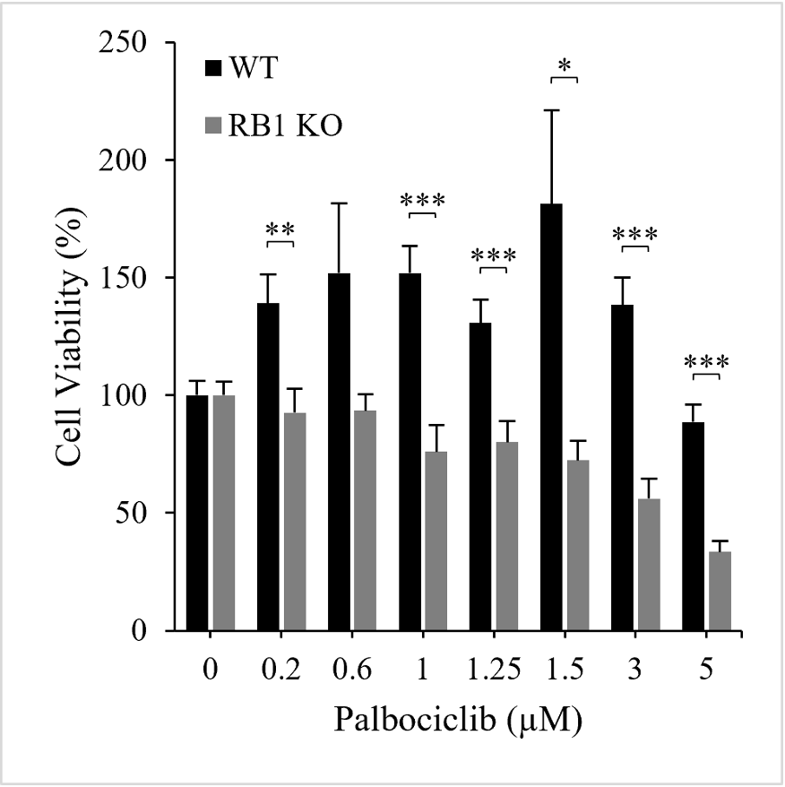
CDK 4/6 inhibitor Palbociclib has been demonstrated an effective immunotherapy in breast and bladder cancers. The therapeutic inhibits cyclin D-CDK4/6 complexes from deactivating RB1 and promoting cell cycle progression. Traditionally having been implemented only for the treatment of RB1-positive tumors, the drug has more recently undergone testing in RB1-deficient tumors. We explored the response of UMUC1 wild type (WT) and RB1 knockout (KO) to Palbociclib with an endpoint assay.
Figure 1. Palbociclib on UMUC1 cell viability (F=6.79; df=15; p<.0001).
Our data were consistent with the hypothesis that KO samples would exhibit increased drug susceptibility (Fig. 1). This examination uniquely isolated RB1 status in CDK 4/6 inhibitor testing and underscored the promise of Palbociclib in novel applications.
Immune ligand RNA expression increased in RB1-deficient BC:The PD-1 pathway mediates body cell recognition by lymphocytes via the connection of a cell-surface PD-L1 ligand with a T-cell PD-1 receptor. The interaction neutralizes immune responses to healthy body cells but may be leveraged by cancerous cells which express PD-L1. Targeting inappropriate ligand expression, treatment with pembrolizumab monoclonal antibody therapy demonstrated successful disruption of the PD-1 pathway in studies of advanced BC. RB1 implication in a related PD-L1 pathway prompted exploration of PD-L1 expression in cases of RB1 deficiency.
Figure 2. Left: CD274 RNA expression by RB1 WT and KO UMUC1 (F=5.36; df=2; p=0.046211). Right: CD274 RNA expression by RB1-deficient 5637 and HT1376 relative to UMUC1 WT control (F=5.19; df=2; p=0.016609).
Through RT-qPCR, we identified increased PD-L1 (CD274) RNA expression in RB1-knockout UMUC1 and two established RB1-deficient cell lines (Fig. 2). These exploratory experiments prompted RB1 and CD274 RNA and protein assessments between more numerous cell lines, though further tests would have been cost prohibitive. Regardless, PD-L1 modulation by RB1 speaks to the therapeutic susceptibility which mutation incurs and should be explored.
RB1 stands a consequential biomarker whose pathways offer therapeutic targets to be exploited. While mutation associates with poorer patient outcomes, it brings vulnerabilities to be leveraged in the development and application of highly selective treatments.
Jenna’s Project
I performed a quantitative polymerase chain reaction (RT-qPCR) to quantify gene expression in bladder cancer cells. This allowed me to compare the relative amounts of RNA expressed between cell lines. Previously, Dr. Craig looked at the difference in FOXA1 expression between WT and RB1 KO UMUC1 with RT-qPCR and western blotting. Her findings supported the hypothesis that FOXA1 gene expression would decrease significantly with the removal of RB1, resulting in a more aggressive and invasive cell line.
My goal was to find and measure the expression of a gene of characteristics like FOXA1. I identified Fibroblast Growth Factor Receptor 3 (FGFR3) as a gene of a comparable profile. Like FOXA1, FGFR3 has CpG islands that are within the introns and exons of the gene. With this information, we hypothesized FGFR3 would also have decreased gene expression in our RB1 KO cell line compared to the WT. FGFR3 instructs the creation of various proteins which play roles in the regulation of cell growth and proliferation. In muscle invasive bladder cancers (like our UMUC1 cell line), FGFR3 mutations and decreased expression are associated with worse prognoses due to their poor reaction to chemotherapy.
I ran qPCR plates RB1 KO F and RB1 KO B cells to compare FGFR3 RNA expression to a WT control. In each plate, I used probes for 18S (a gene expressed in all cells to serve as a control), FOXA1, RB1, and FGFR3. Using FOXA1 as our standard, I analyzed the expression of FGFR3. In RB1 KO cells, FGFR3 and FOXA1 RNA were suppressed in comparison to WT cells.
Figure 1. FGFR3 and FOXA1 RNA expressed by UMUC1 cells. (p=<.0001)
These data underscored the severity of RB1 mutations in BC. RB1 mutations are associated with a poorer patient outcome and can impede patient response to treatment. Witness to FGFR3 suppression elicited by RB1 loss in vitro, we hope to improve understanding of RB1 as a biomarker to help better predict patient responses to therapeutics.
Lena Schaefer, Ben Durham, Salim Alwazir, Van Pham, and Jasper Givens
The students of BK Lab. From top left to bottom right: Van Pham ’24, Ben Durham ’24, Lena Schaefer ’23, Jasper Givens ’25, and Salim Alwazir’24
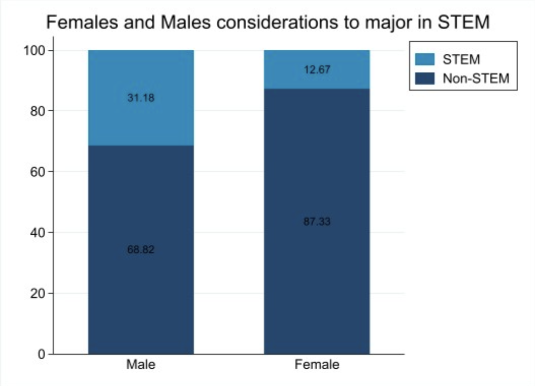
Have you ever walked into a science, technology, engineering, or math (STEM) class only to notice in your class of about twenty (or more) there are only one or two women? Maybe most of your STEM teachers in high school were male. On top of this, maybe you’ve noticed the relative infrequency of female role-models in STEM. Given these common experiences, it isn’t so hard to believe that there aren’t as many women who make it all the way through the STEM education system to STEM careers, or don’t advance as far in their STEM career areas when compared to men. These anecdotal observations may partly explain why women make up only 34% of the STEM workforce. In fact, when looking at survey data from the nationally-representative High School Longitudinal Study (HSLS:09) dataset (Exhibit 1), we see that the number of male students who considered majoring in STEM is almost double that of female students.
Exhibit 1. Tabulation of Student Gender and Students’ Consideration in Majoring in STEM
Perhaps even worse is the fact that this issue has the potential to feed into itself as if women are continually driven away from STEM, there are even fewer female role models for future students. Given this, we want to understand why women leave STEM. Our lab examines possible factors that may influence women’s departure from STEM at the transition from high school to college, within college, and from college to career.
Gender Differences in Preferences over Job Attributes Before and During Careers in STEM
Lena Schaefer ’23
I am a rising senior with an Economics major and a German Studies minor. This is my first summer doing research, and I am working with Professor Blume-Kohout in the Economics department. Last semester I studied abroad in Vienna, Austria and I had such an amazing time, but it feels great to be back on campus for the summer! I am from Atlanta, Georgia so it’s nice to be able to be with other Gettysburg students since I wouldn’t be able to see them if I were working at home and I haven’t seen anyone from school in 6 months. Outside of my academics, I am involved with a few other things on campus. I am on the women’s soccer team, a member of the Chi Omega sorority, and a part of the Garthwait Leadership Institute. One thing I love about being able to do research on campus is that I’m still able to continue the traveling life I have gotten to love from last semester. Over the weekends, I am able to explore new things in and around Gettysburg, along with traveling with other members of X-SIG to further places, such as DC and Baltimore. I was even able to travel to Newport over the Fourth of July weekend and see a place I’ve never visited before.
This summer I am working on research focusing on why there are so few women working in STEM professions. I am focusing more specifically on differences in the importance workers place on specific job attributes by gender, college major, and occupation. For my research I am using data from the 2019 National Survey of College Graduates (NSCG). The survey asks people from ages 75 and under who indicated they received a bachelor’s degree. The NSCG collects extensive employment information such as job status and importance of job attributes, which is the main focus of this research. It also collects information on education, such as all different levels of degrees that were earned by each individual, along with their demographic information. The NSCG is part of an ongoing data collection program through the National Science Foundation, given every two years using the same participants who are still within the age range, and who are still willing to participate. This allows me to compare how preferences for different job attributes have changed, not only across age groups, but also throughout time.
There are hundreds of variables included in the 2019 NSCG data set that I used, so to be able to use them in a way that is relevant to my research, I created new variables from the already existing ones using a statistical software called Stata. Within the data set, there are missing observations which I removed from the data that I ended up using in order to keep my results consistent. After going through all of the variables and observations, I ended up using around 91,000 observations per data set to find the best results to answer my question.
The first research question I am looking into is, within my sample, within each STEM field, is there any evidence of gender differences in importance graduates place on various job attributes. In order to find this answer, using the data set, I ran a regression for each job attribute, split up by field of study, and gender. I also only included participants aged 42 and below. For this question, I am also looking at the difference between various occupations. So far, I have run the regressions and am now working on breaking them down and figuring out the important statistics I was able to find and to include in my results tables.
This Figure shows the results of how likely a female is to say that opportunity for advancement is very important to them compared to men, split up into these individual fields of occupation. To interpret this graph, you must look at where the dots are in relation to the red line, zero. If a dot is very close to the red line, as Biological scientist is in this graph, this means that women in this field are just as likely to say that opportunity for advancement is very important as men are. A dot well above the red line, like Engineer for example, means that women in this field are more likely to say that opportunity for advancement is very important to them. Lastly, a dot below the red line, such as social and related scientists, means that women are less likely to say that the opportunity for advancement is very important to them than men are in this field. The numbers on the side of the graph tell you the percentage points women are more or less likely to say that opportunity for advancement is very important than men. This graph was derived from a table that Stata produced after running regressions with the variables I mentioned earlier. The chart shows the exact numbers, percentage points, and whether or not each result is statistically significant, but the graph shows it in a more visual way.
Eventually, I will be able to answer two more research questions I have. I want to see if, within each gender, is there a significant difference in importance graduates place on various job attributes over time, with age, or in STEM versus non-STEM careers. I also want to know if across STEM occupations, is there any evidence of systematic differences in the importance of various job attributes. After being able to answer these questions, it can help us understand why there are so few women in STEM careers, even though many more women are graduating with STEM degrees.
Pathways Through (or Away From) STEM at the College Level
My name is Ben Durham and I am a rising junior mathematical economics and mathematics double major here at Gettysburg College. This is my second summer of X-SIG research with Prof. Blume-Kohout in the economics department. On campus, I have served as a Peer Learning Assistant (PLA) and grader in the math department, and I look forward to working as a PLA again this coming academic year in the math department and the economics department! Outside of my academic interests, I enjoy going to the gym and I compete in powerlifting, so I have a tangential interest in research about strength training and nutrition.
This summer, I’m working on improving our understanding of undergraduate students’ transitions to and from STEM. Understanding why people transition away from STEM majors at the undergraduate level may be useful in determining what could be changed to influence students retention, especially for currently underrepresented groups. Depending on the prevalence of this phenomenon in our sample, I may also be able to study some of the factors associated with switching from non-STEM majors into STEM majors.
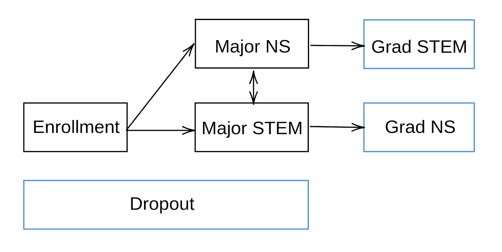
To understand these transitions, I make use of a dataset from a large, public, minority serving institution tracking 16,116 students enrolled at this institution from fall 2006 to fall 2015. The data include a student’s declared major over time, any STEM courses a given student takes during their time of enrollment, and several covariates including demographic information, socioeconomic background, and indicators of ability including high school GPA and SAT or ACT students where available. This dataset is unique in its demographic composition, specifically the proportion of Hispanic students. This sample consists of about 40.32% Hispanic students, despite Hispanic students making up only 15% of enrolled college students in 2010. From this data, I can construct a timeline for each student, beginning at enrollment and going through intermediate states such as major declarations until reaching an absorbing state such as graduation or dropout.
The figure above shows the states I identify in the dataset and possible transitions from intermediate states (outlined in black) to absorbing states (outlined in blue). I use the abbreviation “NS” as a shorthand for “Non-STEM.” To avoid cluttering the diagram, I omit arrows from the intermediate states to Dropout since a student can transition from any of the intermediate states to Dropout.
Some of the key transitions we would like to understand include the two-way transition between Major STEM and Major NS and the transition between Major STEM and Grad STEM. Examining factors associated with making either transition between Major STEM and Major NS will help us understand what might influence a person already in STEM to leave STEM or what might draw someone into STEM. Examining the transition between Major STEM and Grad STEM will help to understand factors associated with completing a degree for students who are already majoring in STEM.
I will use a competing risks model to identify what factors may play a role in altering students’ trajectories. In this context, the absorbing states Grad STEM, Grad NS, and Dropout are “competing risks” since once an individual enters one of these states, they are no longer “at risk” of transitioning to any of the other states. Some key factors I will consider include instructor race-matching and gender-matching (meaning when the instructor’s race or gender is matched to the student’s race or gender) and classroom gender composition in STEM courses. Conceivably students may be more likely to continue in a field if they have potential role models in the form of instructors of the same race or gender or if they are surrounded by peers that are like them in their degree program. As mentioned, this dataset contains a significant proportion of Hispanic students, which will make it possible to understand race-matching effects which would be much more difficult to do with precision in a dataset containing a more typical proportion of Hispanic students. Additionally, this may allow me to study the even rarer case of simultaneous race and gender matching for non-white students.
Thus far, I have cleaned and transformed the data into the format required to estimate a competing risks model. Competing risk models require the data be formatted such that there is one observation per individual per time period that the individual is “at risk” of transitioning into one of our states of interest. In our case, this means one observation per semester prior to a student graduating with his or her first bachelor’s degree or dropping out. I investigate cases such as students missing information for key variables to identify patterns among these students to explain why their data may not look as I would expect.
Having reconciled most of the outstanding issues with the dataset, the next step is to specify the model or models I will use to understand these transitions, run these models, and then communicate these results in a paper. This is what will occupy me for the remainder of my research this summer.
The Gender Gap in STEM Fields: The Period of High School into College
We are Van Pham and Salim Alwazir, we are both rising juniors at Gettysburg College majoring in Mathematical Economics and minoring in Data Science. We are also both international students: Van from Vietnam and Salim from Palestine. This summer we are working together on a research project for Professor Blume-Kohout. It’s very fortunate to have a lot of students doing X-SIG this summer, so the social life is not much different from during the year. In her free time, Van hangs out with her friends and cooks some good food. She also studies some courses from DataCamp to learn statistics and coding in R to better prepare for the next year at Gettysburg. Salim enjoys hanging out with his friends and visiting cities around the U.S. He also enjoys using online platforms such as Udemy and Coursera to learn and sharpen his technical skills. This is our first research experience in economics and we are very excited to share our work with you. Also, neither of us has used Stata to perform statistical analysis and build regression models before, so it is a new and valuable experience. Furthermore, we both feel excited about how this research can contribute to a lot of change on campus and hopefully nationally.
We are working on understanding the gender gap in STEM (Science, Technology, Engineering, and Mathematics) fields in the period between high school and college. Our work includes data cleaning, statistical analysis, and estimating relationships between variables. We are aiming to understand the gender gap in STEM by exploring the student-teacher interaction, student achievements, and the student’s classroom experience in high school and college.
We started our work by summarizing multiple research papers and prior literature to develop a general idea of our research questions and hypothesis, as well as the variables we want to extract from the dataset. The dataset we are using is the High School Longitudinal Study: 2009 (HSLS:09). The datasetincludes over 10,000 variables and information about more than 25,000 students from 940 different schools across the United States. In Fall 2009, the HSLS:09 surveyed 9th grade students (base year), parents, math and science teacher, administrators, and counselors, then followed up with the student respondents three times: in Spring 2012 (11th grade), Summer and Fall 2013 (after most graduated from high school), and in 2016 (about 3 years after high school graduation). Finally, between Spring 2017 and Fall 2018 (about 4 years after high school graduation), the survey collected college transcripts for students who attended college. Our study focuses on responses from the students, math and science teachers, and parents.
For the first three weeks of the summer, we looked into the variables and chose which variables we wanted to use. We had a lot of discussions (and maybe some arguments, too). But overall, we have some very good results, and a lot of new ideas that we exchange with each other. From the variables and from the inspirations of some articles we read as well as the professor’s suggestions, we chose to focus on three possible outcomes (considering majoring in STEM, declared STEM major in college, and completed STEM majors), and investigate how the targeted variables relate to our outcome. Examples of these variables are Science/Math teacher beliefs about who is better in Math/science, students’ beliefs about who is better in Math/science, whether the teacher listens to students’ ideas, whether the teacher treats men and women differently, and other variables to understand which factors have a significant impact on our outcomes.
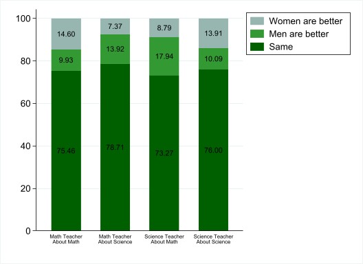
We are currently looking into replicating the framework of Dario Sansone, who was mainly looking into the relationship between high school student’s beliefs about female abilities in math and science and their teacher’s gender, beliefs, and classroom behaviors. He found that these formed beliefs are related to the decisions by female students to take advanced math and science classes in Sansone’s 2019 paper. We are building on his framework to investigate how all the previously mentioned factors might affect a female student’s decision to major in STEM, and their probability of completing a STEM degree. We use Stata, a general-purpose statistical software package to test for statistical significance and to estimate regression models, and we have envisioned a plan on how we want to design our models. While working, we have found many interesting things to consider. For example, most teachers believe that women and men have the same abilities in math and science. On the other hand, there are some gendered beliefs that are interesting to explore. For instance, the percentage of math teachers who believe that women are better than men in math is higher than the percentage of math teachers who believe that men are better. However, the percentage of math teachers who believe that women are better in science is lower than the percentage of math teachers who believe that men are better in science. Additionally, the percentage of science teachers who believe that women are better in science is higher than the percentage of science teachers who believe that men are better in science. However, the percentage of science teachers who believe that women are better in math is lower than the percentage of science teachers who believe that men are better in Math (Figure 1). We can conclude that teachers tend to think that women are better in their field of expertise, but overall have a stereotype that men are better in the field they are not teaching. This informs us that there is a gendered stereotype that men are better at science/math, but the experts in the field state otherwise! Therefore, we are aiming at studying how these beliefs and teacher behavior in the class affects female intentions to major in STEM.
Next steps will include building our regression model to estimate the effect of the chosen variables on female students declaring and completing a STEM degree. Also, we will be writing our data section where we will explain our key variables and provide some insights about the descriptive statistics, which inform initial results.
The Impact of Values on STEM Interest and Careers
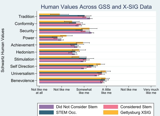
Hi, I’m Jasper Givens and I am currently a rising sophomore. Outside of school I enjoy playing the guitar, making video essays, and hiking in my home state of Washington. I am majoring in Mathematical Economics and Computer Science and hope to become a machine learning engineer after college. This summer I am working with Professor Blume-Kohout of the economics department on researching the values of people in STEM occupations and undergraduate programs. My research is composed of two main parts: data from the 2012 General Social Survey, and my own research experiment conducted at Gettysburg over the summer.
Why does it matter?
According to the American Action Forum, the U.S. will be 1.1 million STEM workers short in 2024. This vital profession group includes scientists, engineers, statisticians and computer scientists. Due to the importance of these groups to the economy, and the increasing need for STEM workers, it is necessary to understand the differences between STEM workers and the general population. Furthermore, STEM careers are some of the worst in terms of gender disparity; women are especially underrepresented in non-life science STEM careers. By investigating the values of STEM workers, we hope to provide information which will allow teachers, professors, and policy makers to better understand how to develop a strong and diverse STEM workforce.
How do we measure values?
In order to measure the characteristics of STEM majors, it was first necessary to establish a metric by which to measure STEM and non-STEM individuals. For this purpose, I am using the Portrait Value Questionnaire (PVQ) instrument first described by Shalom Schwartz in 2002. The PVQ is based on Schwartz’s theory of human values, a system which contains 10 human values which Schwartz theorizes all human cultures share to some extent. The original version of the PVQ contains 40 questions with 4 questions each corresponding to one value. This allows for a consistent measurement of each of the 10 values.
Below is a diagram depicting the 10 Schwartz Human Values. They are organized by their relationship to each other such that adjacent values are more closely related while opposite values are at odds with each other. The test uses a 6-point Likert scale which ranges from “very much like me” to “not like me at all”. Across various experiments, Universalism and Benevolence are usually the highest while Power and Achievement are usually the lowest. You can take the PVQ yourself here.
Figure 1: The 10 Schwartz human values displayed graphically
The 2012 General Social Survey Data
The 2012 GSS contained the PVQ21, a shortened (21 question) version of the original PVQ. The survey also asked whether participants had ever considered a career in science or in engineering, and about their current occupation. Using these variables, I ran linear regressions on the normalized mean of each of the 10 values with career category (never considered STEM, considered STEM, in STEM career) as the dependent variable. The data points from these regressions were used to perform t-test comparisons, which gives the probability that the difference exists given that the independent and dependent variables are uncorrelated. Self-Direction was found to be higher amongst those who considered STEM careers and those who are currently in STEM careers, while Security and Tradition were lower in those same groups.
What about students at Gettysburg?
For the second part of my research, I administered the PVQ21 to X-SIG students and faculty mentors at Gettysburg College. Students participating in the X-SIG program are usually STEM majors. I am using these data to see if the values most strongly held among STEM students at Gettysburg follow the same pattern as STEM workers in the GSS data.
Below are the results of this work so far, comparing the responses of Gettysburg X-SIG students to those from the General Social Survey.
Figure 2: Schwartz Human Values in GSS and Gettysburg X-SIG respondents
For the remainder of the summer, I will conduct further research on the Gettysburg X-SIG data. Existing literature has shown that men and women on average place importance on different human values; however, this difference has decreased over time. I will examine the relationship between men and women in STEM fields in my data. In doing so I hope to establish whether differences in human values can explain some of the gender disparity in STEM occupations.
Hello from Dr. Presser team! This summer we are making games using Procedural Content Generation (–PCG). To understand more about a game using PCG I will provide some background information to help readers to understand.
PCG can be used in Role Playing Games, games in which players play in the role of characters in fictional settings. Some example of RPGs are Dungeons and Dragons, Final Fantasy, World of Warcraft, …
In this article I will focus on make an RPG using PCG. There are three main steps to create an RPG:
The first step is to create a map or space of the game. A map or space can include paths, building, or any kind of space that a player can move or go around. For instance, if our RPG is about Pirate History then our map will be ocean that helps player move among islands in the ocean.
Second step is to create missions, or quests for each location of the game and connect missions in an appropriate way. In other words, missions are tasks that player need to do or solve to make progress in the game. Keeping with previous Pirate game as an example, a mission can be a player buying a ship to defeat other pirates to collect treasures.
The last step is to combine the map and the missions in such a way that game can play without any errors.
At the moment we finished making a functions for the player and almost finished creating the map for our game.
The image above is the whole picture of our map for our game. Our map was created by using cellular automata. This is the link for anyone who want to understand more about cellular automata. I found that this articles explained quite careful. https://mathworld.wolfram.com/CellularAutomaton.html
The image above is a picture that present the game from the view of the player. In the picture, there are two spider-monsters that are hunting the player. Defeating these monsters will the first tasks the player need to do to in this game.
Our task in the future is to create more and more quests and missions, and then connect them together to make a complete game.
Hello everyone, My name is Sebastian Gibbs and I am a rising senior at Gettysburg College. I am a physics major from Bethlehem, PA and I am conducting my research with Dr. Ryan E Johnson. This is my first year conducting research for X-Sig at Gettysburg College, and it has been going very well so far. Along with this being my first time doing research, this is also my first time coding which has been a challenge, but I have been developing and learning everyday which has enhanced my skill set. My research is a continuation of Sheldon Johnson’s research who graduated last year from Gettysburg (Class of 2022). My research deals with the gravitational aspect of time dilation as proposed by Albert Einstein’s Theory of General Relativity. This has led me to model the first direct dynamical detection of a dual supermassive blackhole system at sub-kiloparsec separation. General relativity is a concept that involves the curving or warping of space from the invisible force that we interact with daily. The theory of General Relativity is founded on the idea that massive objects cause a distortion in space time which leads to the subject of time dilation. In physics and relativity, time dilation is recognized as the slowing of time perceived by one observer compared to another, depending on their relative motion. Along with this, time dilation can also be affected by gravity which is the spark of motivation for this project. In my research with Professor Johnson, we are attempting to replicate the dual supermassive blackhole system (Voggel,2022) using three-dimensional visualizations on a computer software program which is named python in order to visually perceive time dilation. The overall goal for this project is to observe paths of constant time through intersecting gravitational fields.
Figure I of creating the Dual Blackhole System
Here is one of the first three-dimensional visualizations that me and Dr. Johnson have created from the data that we collected about the blackhole system from the constellation NGC 7727 which is approximately 89 million light years away. This was the first blackhole that we replicated and coded into python. The initial goal for this was to create a perfectly spherical object with the data we obtained about the blackhole system. In order to perform this we had to code in the X,Y, and Z spherical coordinates and develop a random number generator to select various positions on the sphere within the three-dimensional grid everytime we ran the cell. We also implemented a modified version of The Schwarzschild Equation into the cell in order to view the time dilation within the replicated sphere. In order to view the time dilation within the coded sphere we had to adjust the amount of contours that appeared, and choose a specific color scale that best represents the amount of contours as well. The contours within the 3d figures are the different shades of color that transition inside of the sphere as it approaches its core. The side color scale bar guides the reader to understand the different intensities of time dilation that is apparent within the sphere. As we can see above (Figure 1), the time dilation transitions from low intensity (Outer shell of the sphere) to very high intensity (the glowing yellow in the middle) which shows how time is being affected from the gravitational field of the blackhole. As the contours approach the core of the sphere, time continuously slows down. Once we got to the point where the sphere appeared to be like the figure above, we moved on to replicating another blackhole within python to truly create the dual supermassive blackhole system.
Figure II of creating the Dual Blackhole System (View from the X coordinate)Figure III 3d visualization from the Y coordinate
The existence of stellar-mass binary black holes was discovered in the year 2015 which makes this a fairly new phenomenon in the astrophysics field. Most black holes usually have masses between three and ten solar masses which makes these specific black holes astounding. These discovered merging black holes are approximately 30 solar masses each and about 1.3 billion light years away. The reason why these black holes were able to be detected is because of LIGO (Laser Interferometer Gravitational-Wave Observatory) which observed the gravitational wave signature of the two merging black holes (Caltech, 2022).
In this past week, Professor Johnson and I have modeled the first, and newly discovered, dual supermassive blackhole system (See Figure 2 and 3). While creating this visualization, we calculated the mass ratio between the two black holes in the system. The smaller blackhole which is visualized in the color purple is approximately 6.33×10^6 solar masses (a solar mass is the mass of the Sun, ~2e30 kg). The larger blackhole in the 3d visualization is approximately 1.54 ×10^8 solar masses. Most galaxies, including our own Milky Way Galaxy, contain supermassive black holes which can reach up to millions or billions of solar masses.
We calculated the Schwarzchild radius of each black hole in the binary system, and we were able to compute this by using The Schwarzchild radius equation which is (Cosmos, 2022). Because our simulation space was not large enough to encompass the astronomical units of the positional data, and in an effort to faithfully reproduce the size and relative positions of these supermassive black holes, we used the black hole diameters (specifically the larger black hole’s diameter) as a scale for expressing the separation distance between the two. Since the larger supermassive black holes radius was 2.83 x 10^8 miles, and the separation distance was 9.58 x 10^8 miles, then the seperation distance measured in black hole diameters is approximately 3.38. We can observe this separation distance in the figure below.
Figure IV, Separation distance of approximately 3.38 large black hole diameters within the 3d grid.
Now comparing the masses of the first detected binary system to the binary system that Professor Johnson and I are researching is astonishing. If we take the mass of the smaller blackhole in our research (6.33×10^6 solar masses) and compared it to one of the detected black holes from 2015 ( 30 solar masses) we would see that the smaller blackhole that we are researching is approximately 211,000 times as massive as one of the discovered black holes in the first binary system. In calculating the mass ratio of the black holes in our research, we found that the larger black hole in NGC 7727 is around 25 times more massive than the other blackhole. We coded this calculation into python which then created this size difference within the 3d grid (See Figure 2). We also changed the color scheme in this visualization in order to enhance the perspective of time dilation within the blackhole system. The next step for this research project is to find a constant path of time around the time dilation in the 3d grid.
Along with having to code for most of the day, Dr. Johnson has established a mandatory hacky sack session daily in order for us not to be stuck inside for all eight hours. Since the start of summer research, I believe it is safe to say that my hacky sacking skills have developed pretty well along with my fellow research partners within the Johnson lab. Dr. Johnson has made multiple connections with hacky sacking and life lessons which I believe is pretty common since I hear about them every year from past researchers who have worked with him. The one connection that will stick with me from hacky sacking is having the ability to stay consistent. This idea of consistency comes from the daily act of performing this activity. The more consistent someone is, the more development and growth they will see and receive. This is also true on the coding side of things. As I have stayed consistent with coding everyday at work, I have noticed a lot of development and improvement in this activity as well.
I have enjoyed my research experience so far with Dr. Johnson, and I expect this level of enjoyment to rise from this point on. Dr. Johnson has been my mentor, and advisor since my freshman year and we have always had a strong connection and understanding with one another. Working with Dr. Johnson has allowed me to expand my knowledge about physics and develop an abstract way of thinking. He also has the ability to teach in a versatile manner which allows students from any background to develop and understand the subject that is being taught. I’m very grateful for this opportunity to explore time dilation and special relativity since it will allow physicists like myself to be able to understand gravity, time, and space in an advanced manner. This research can potentially create paths for future space travel. Creating visual projections of these massive entities along with astronomical space data may dispense a plan for future celestial expeditions.
111Voggel, K. T., Seth, A. C., Baumgardt, H., Husemann, B., Neumayer, N., Hilker, M., Pechetti, R., Mieske, S., Dumont, A., & Georgiev, I. (2022). First direct dynamical detection of a dual supermassive black hole system at sub-kiloparsec separation. Astronomy & Astrophysics, 658. https://doi.org/10.1051/0004-6361/202140827
Hi! I am Thanh Duong from Professor Presser’s lab. Like my other two labmates, this summer, I will be working on making a game. This is my first time doing X-SIG and research in general, and I have enjoyed it a lot so far.
About my project: I will be working on a variant of the game tic-tac-toe. The game will be played in the icosahedron shape (20 faces in three dimensions). Two players will be competing with each other; each player will be able to play both O and X; the person getting the first path of 4 of either O or X will win the game. To make the game more interesting, some of the faces of the shape will be blocked randomly (more specifically, for most of the time, about 3 or 4 faces will be blocked), meaning that the board will be different each time we play. I also create the One-player mode, meaning that the player can choose to play with the computer at different levels (Easy – Medium – Hard).
Methods: My first step was to determine the optimal “content” of the game, which are “how many to win” and “how many to block”. For this, I created a computer player with simple rules: win an immediate win, avoid an immediate loss, and play randomly otherwise. I then let them play with each other to collect the statistics: the percentage of Player 1 winning/losing/tied, and the average number of moves for the game to end. I then choose the “content” with the best the statistics (I want the percent of Player 1 winning/losing to be close to each other as I don’t want my game to be biased, while choosing the best percentage of tied games and the average number of moves were kind of subjective).
My next step would be to create a computer player for the One-player mode. Since I want to have different levels of difficulty, I use neural networks as the size of the neural networks would be correlated with how “smart” they would be. I first simulate a large number of games, storing each state of the games, with each state being marked with the final result of a match. I use that for the neural network to learn. Then, for each computer move, for every possible move, I use the simulated results to produce the next state of the game and use the model to predict the outcome. I will use the move with the most favorable outcome for computer play as its next move.
My last step, with I have not started yet, is to finish the interface. I will use the game engine Godot for this task.
My experience: It has been a great journey! I am learning new things every day, whether from the professor, from reading articles, or from mistakes I made when writing codes. I really like that for making games, I do not focus on a specific field like class projects only, but on a much broader field.
As you can see, my project involves a lot of simulating and building models, which could be faster when running on several machines. Below is a sneak peek of how “A day in my lab” looks like: